Forward Kinematic
A foundation capability enabling robots to interact reliably with their environment is the ability to compute where each part of the mechanism will be, given a set of joint inputs. This process, known as forward kinematics, underpins everything from basic motion visualization to advanced trajectory planning. In this tutorial, we'll explore the mathematical framework and practical implementation strategies that allow you to determine an end-effector's pose (position and orientation) in space, given the configuration of its joints.
Problem
At its core, forward kinematics is the problem of mapping joint space, the vector of actuator or joint variables, to Cartesian space, the spatial pose of a robot's link or end-effector.
This is achieved by using the DH parameters to compute a homogeneous transform matrix that is dependent on a joint state. Recall that a homogeneous transform is defined as:
$$ T=\left\lbrack \begin{array}{ccccc} & & & | & \newline & R\in {\mathbb{R}}^{3\textrm{x3}} & & | & t\in {\mathbb{R}}^{3\textrm{x1}} \newline & & & | & \newline -- & -- & -- & + & --\newline 0 & 0 & 0 & | & 1 \end{array}\right\rbrack =\left\lbrack \begin{array}{cccc} r_{11} & r_{12} & r_{13} & \Delta \;x\newline r_{21} & r_{22} & r_{23} & \Delta \;y\newline r_{13} & r_{32} & r_{33} & \Delta \;z\newline 0 & 0 & 0 & 1 \end{array}\right\rbrack $$
The goal is to compute a transformation matrix that is only depending on the actuator variable q:
$$ T\left(q\right)=\left\lbrack \begin{array}{ccccc} & & & | & \newline & R\left(q\right) & & | & t\left(q\right)\newline & & & | & \newline -- & -- & -- & + & --\newline 0 & 0 & 0 & | & 1 \end{array}\right\rbrack $$
These transformation matrices define the translation and rotation from two consecutive joints. Concatenating them lets us compute the pose of a series of links up to the end-effector.
Consider the Universal Robots UR3. Since all joints are revolute, the joint variables q_i are assigned to the theta parameter in the DH table below:
syms q1 q2 q3 q4 q5 q6 real
DH=[ %by Universal Robots (website)
   %a       alpha       d       theta
   0        pi/2        0.1519  q1;
   -0.24365 0           0       q2;
   -0.21325 0           0       q3;
   0        pi/2        0.11235 q4;
   0        -pi/2       0.08535 q5;
   0        0           0.0819  q6;
    ];
Using the Symbolic Math Toolbox we can transform these DH parameters into a homogeneous transform matrix depending on the jointstate q.
Symbolic Math Toolbox
To model the Robot using the Symbolic Math Toolbox, we need to define Transform matrices using symbolic variables. We can later substitute with real values to compute the Cartesian pose of a series of links.
DH to Homogeneous Transform
Lets understand how to construct a homogeneous transform matrix from the DH parameters.
Remind that the DH parameters describe the kinematics of a robot's manipulator by defining the relative position and orientation of each adjacent link. They are summarized by four parameters:
- θ (theta) → Joint angle (rotation around z_i-1 to go from x_i-1 to x_i) → used for revolute joints.
- d → distance along the z_i-1 between x_i-1 and x_i → used for prismatic joints.
- a → distance along the x_i between z_i-1 and z_i
- α (alpha) → angle between z_i-1 and z_i from x_i
Basically, the DH modeling transformation involves two translations and two rotations, performed in the following order:
- Rotation around Z, aligning the common normals (X-axis) using theta (using DH parameter \(\theta \;\), for revolute joints this is the input q).
- Translation along the Z-axis, placing the origins in the same point. (using DH parameter d, for prismatic joints this will be input q)
- Translation along the X-axis, placing the origins in the same Y-Z plane (using DH parameter a).
- Rotation around X-axis, aligning both Z-axis. (using DH parameter \(\alpha\) )
FirstRotation =
syms alpha theta a d real %setup symbolic variables and define them as real

FirstRotation=trotz(theta) %create a homogeneous transformation matrix -->Rotate around z axis
$$ \displaystyle \left(\begin{array}{cccc} \cos \left(\theta \right) & -\sin \left(\theta \right) & 0 & 0\newline \sin \left(\theta \right) & \cos \left(\theta \right) & 0 & 0\newline 0 & 0 & 1 & 0\newline 0 & 0 & 0 & 1 \end{array}\right) $$
FirstTranslation=transl([a 0 0]) %create a homogeneous transformation matrix --> Move along x axis
$$ \displaystyle \left(\begin{array}{cccc} 1 & 0 & 0 & a\newline 0 & 1 & 0 & 0\newline 0 & 0 & 1 & 0\newline 0 & 0 & 0 & 1 \end{array}\right) $$
SecondTranslation=transl([0 0 d]) %create a homogeneous transformation matrix --> move along z axis
$$ \displaystyle \left(\begin{array}{cccc} 1 & 0 & 0 & 0\newline 0 & 1 & 0 & 0\newline 0 & 0 & 1 & d\newline 0 & 0 & 0 & 1 \end{array}\right) $$
SecondRotation=trotx(alpha) %create a homogeneous transformation matrix -->rotate around x axis
$$ \displaystyle \left(\begin{array}{cccc} 1 & 0 & 0 & 0\newline 0 & \cos \left(\alpha \right) & -\sin \left(\alpha \right) & 0\newline 0 & \sin \left(\alpha \right) & \cos \left(\alpha \right) & 0\newline 0 & 0 & 0 & 1 \end{array}\right) $$
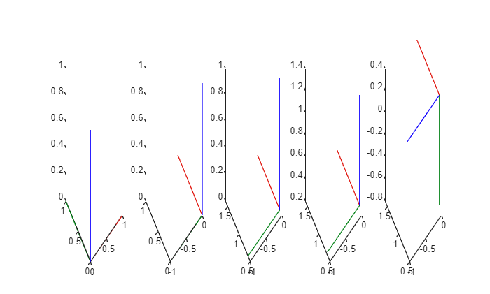
Let us visualize what is happening with each of these transforms.
Consider this arbitrary set of DH parameters:
          % a      alpha     d          theta
DHexample=[0.6,    -pi/2,    0.24,      pi/2]
DHexample = 1x4
    0.6000   -1.5708    0.2400    1.5708
See how each step is multiplied with the previous transformation:
                                % Input matrix      variable    value
exampleFirstRotation =      subs(FirstRotation,     theta,      DHexample(4));
exampleFirstTranslation =   subs(FirstTranslation,  a,          DHexample(1));
exampleSecondTranslation =  subs(SecondTranslation, d,          DHexample(3));
exampleSecondRotation =     subs(SecondRotation,    alpha,      DHexample(2));

M=zeros(4,4,5);
M(:,:,1)=eye(4);
M(:,:,2)=M(:,:,1)*double(exampleFirstRotation);
M(:,:,3)=M(:,:,2)*double(exampleFirstTranslation);
M(:,:,4)=M(:,:,3)*double(exampleSecondTranslation);
M(:,:,5)=M(:,:,4)*double(exampleSecondRotation);

figure;
axis(2*[-1,1,-1,1,-1,1])
for i=1:5
subplot(1,5,i)
plotTransforms(M(1:3,4,i)',tform2quat(M(:,:,i)))
end
Following these steps will result in a homogeneous transformation matrix that concatenates all the DH parameters. We will call these transformation matrices \(A_{\textrm{source}\;\textrm{link}\to \textrm{target}\;\textrm{link}}\). Using the Symbolic Toolbox we can setup a template as:
Ai=FirstRotation*FirstTranslation*SecondTranslation*SecondRotation
$$ \displaystyle \left(\begin{array}{cccc} \cos \left(\theta \right) & -\cos \left(\alpha \right)\,\sin \left(\theta \right) & \sin \left(\alpha \right)\,\sin \left(\theta \right) & a\,\cos \left(\theta \right)\newline \sin \left(\theta \right) & \cos \left(\alpha \right)\,\cos \left(\theta \right) & -\sin \left(\alpha \right)\,\cos \left(\theta \right) & a\,\sin \left(\theta \right)\newline 0 & \sin \left(\alpha \right) & \cos \left(\alpha \right) & d\newline 0 & 0 & 0 & 1 \end{array}\right) $$
or manually set it as:
Ai_symbolic = [
                  cos(theta)     -sin(theta)*cos(alpha)    sin(theta)*sin(alpha)     a*cos(theta);
                  sin(theta)     cos(theta)*cos(alpha)     -cos(theta)*sin(alpha)    a*sin(theta);
                  0              sin(alpha)                cos(alpha)                d;
                  0              0                         0                         1
              ]
$$ \displaystyle \left(\begin{array}{cccc} \cos \left(\theta \right) & -\cos \left(\alpha \right)\,\sin \left(\theta \right) & \sin \left(\alpha \right)\,\sin \left(\theta \right) & a\,\cos \left(\theta \right)\newline \sin \left(\theta \right) & \cos \left(\alpha \right)\,\cos \left(\theta \right) & -\sin \left(\alpha \right)\,\cos \left(\theta \right) & a\,\sin \left(\theta \right)\newline 0 & \sin \left(\alpha \right) & \cos \left(\alpha \right) & d\newline 0 & 0 & 0 & 1 \end{array}\right) $$
Using this symbolic matrix lets us easily substitute different DH parameters to compute the transforms between two consecutive frames.
For the UR3 the resulting matrices are:
A01 = subs(Ai_symbolic, [a alpha d theta], DH(1,:))
$$ \displaystyle \left(\begin{array}{cccc} \cos \left(q_1 \right) & 0 & \sin \left(q_1 \right) & 0\newline \sin \left(q_1 \right) & 0 & -\cos \left(q_1 \right) & 0\newline 0 & 1 & 0 & \frac{1519}{10000}\newline 0 & 0 & 0 & 1 \end{array}\right) $$
A12 = subs(Ai_symbolic, [a alpha d theta], DH(2,:))
$$ \displaystyle \left(\begin{array}{cccc} \cos \left(q_2 \right) & -\sin \left(q_2 \right) & 0 & -\frac{4873\,\cos \left(q_2 \right)}{20000}\newline \sin \left(q_2 \right) & \cos \left(q_2 \right) & 0 & -\frac{4873\,\sin \left(q_2 \right)}{20000}\newline 0 & 0 & 1 & 0\newline 0 & 0 & 0 & 1 \end{array}\right) $$
A23 = subs(Ai_symbolic, [a alpha d theta], DH(3,:))
$$ \displaystyle \left(\begin{array}{cccc} \cos \left(q_3 \right) & -\sin \left(q_3 \right) & 0 & -\frac{853\,\cos \left(q_3 \right)}{4000}\newline \sin \left(q_3 \right) & \cos \left(q_3 \right) & 0 & -\frac{853\,\sin \left(q_3 \right)}{4000}\newline 0 & 0 & 1 & 0\newline 0 & 0 & 0 & 1 \end{array}\right) $$
A34 = subs(Ai_symbolic, [a alpha d theta], DH(4,:))
$$ \displaystyle \left(\begin{array}{cccc} \cos \left(q_4 \right) & 0 & \sin \left(q_4 \right) & 0\newline \sin \left(q_4 \right) & 0 & -\cos \left(q_4 \right) & 0\newline 0 & 1 & 0 & \frac{2247}{20000}\newline 0 & 0 & 0 & 1 \end{array}\right) $$
A45 = subs(Ai_symbolic, [a alpha d theta], DH(5,:))
$$ \displaystyle \left(\begin{array}{cccc} \cos \left(q_5 \right) & 0 & -\sin \left(q_5 \right) & 0\newline \sin \left(q_5 \right) & 0 & \cos \left(q_5 \right) & 0\newline 0 & -1 & 0 & \frac{1707}{20000}\newline 0 & 0 & 0 & 1 \end{array}\right) $$
A56 = subs(Ai_symbolic, [a alpha d theta], DH(6,:))
$$ \displaystyle \left(\begin{array}{cccc} \cos \left(q_6 \right) & -\sin \left(q_6 \right) & 0 & 0\newline \sin \left(q_6 \right) & \cos \left(q_6 \right) & 0 & 0\newline 0 & 0 & 1 & \frac{819}{10000}\newline 0 & 0 & 0 & 1 \end{array}\right) $$
Composing these Transforms lets us find more complex transforms between a series of frames. To get the transformation between frame 0 and frame 2 we can simply multiply A01 and A12:
A02=A01*A12
$$ \displaystyle \left(\begin{array}{cccc} \cos \left(q_1 \right)\,\cos \left(q_2 \right) & -\cos \left(q_1 \right)\,\sin \left(q_2 \right) & \sin \left(q_1 \right) & -\frac{4873\,\cos \left(q_1 \right)\,\cos \left(q_2 \right)}{20000}\newline \cos \left(q_2 \right)\,\sin \left(q_1 \right) & -\sin \left(q_1 \right)\,\sin \left(q_2 \right) & -\cos \left(q_1 \right) & -\frac{4873\,\cos \left(q_2 \right)\,\sin \left(q_1 \right)}{20000}\newline \sin \left(q_2 \right) & \cos \left(q_2 \right) & 0 & \frac{1519}{10000}-\frac{4873\,\sin \left(q_2 \right)}{20000}\newline 0 & 0 & 0 & 1 \end{array}\right) $$
To find the position of frame 2 at the configuration [0, 0] we can substitute:
A02_configuration = subs(A02, [q1,q2], [0,0])
$$ \displaystyle \left(\begin{array}{cccc} 1 & 0 & 0 & -\frac{4873}{20000}\newline 0 & 0 & -1 & 0\newline 0 & 1 & 0 & \frac{1519}{10000}\newline 0 & 0 & 0 & 1 \end{array}\right) $$
You can view it as a decimal with n decimals as:
n=4;
A02_config_decimal = vpa(A02_configuration, n)
$$ \displaystyle \left(\begin{array}{cccc} 1.0 & 0 & 0 & -0.2436\newline 0 & 0 & -1.0 & 0\newline 0 & 1.0 & 0 & 0.1519\newline 0 & 0 & 0 & 1.0 \end{array}\right) $$
Using this composition we can compute the end-effector position when concatenating:
A06 = A01 * A12 * A23 * A34 * A45 * A56;
A06_config=vpa(subs(A06,[q1,q2,q3,q4,q5,q6],[0,0,0,0,0,0]),4)
$$ \displaystyle \left(\begin{array}{cccc} 1.0 & 0 & 0 & -0.4569\newline 0 & 0 & -1.0 & -0.1943\newline 0 & 1.0 & 0 & 0.06655\newline 0 & 0 & 0 & 1.0 \end{array}\right) $$
Robotic System Toolbox
Load a predefined robot or set it up yourself.
ur3=loadrobot("universalUR3", "DataFormat", "column");
You can get the transformation matrix using the getTransform() function.
Use it by giving the following inputs:
- RigidBodyTree Structure (robot)
- Joint Configuration (depending on your data format it is a row/column vector or a structure)
- Target Link name
- Source Link name
A06_RS_toolbox = getTransform(ur3, [0;0;0;0;0;0], "wrist_3_link", "base")
A06_RS_toolbox = 4x4
1.0000    0.0000   -0.0000   -0.4569
    0.0000   -1.0000   -0.0000   -0.1124
   -0.0000         0   -1.0000    0.0666
         0         0         0    1.0000
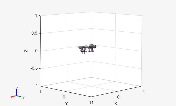
We can visualize a configuration in MATLAB as
figure;
show(ur3,[0;0;0;0;0;0]);
Or display it in ROS using the prebuild function JointStatesToRviz().
To start Rviz:
StartTutorialApplication('Rviz','model','ur3e');
%StartTutorialApplication('Rviz','model','ur3e', 'docker',false); %use this
%when using a native ROS workspace
JointStatesToRviz([0;0;0;0;0;0],'ur3');