Exercise 4.2 - Effort-Based Control using the Dynamic Model
In this exercise, you will implement a joint-space PD controller with gravity and dynamic compensation for a UR manipulator. The goal is to drive all joints of the robot smoothly toward a desired configuration (qd) while respecting joint torque limits.
Task
Your controller will operate in the effort control mode, meaning it will directly send joint torques to the simulated robot.
At each control step, you will:
- Read the current joint positions and velocities from the simulator.
- Compute the dynamic model of the robot (mass matrix, Coriolis/centrifugal terms, and gravity torques).
- Calculate the control torques using a PD law in the joint space.
- Apply torque saturation to stay within physical actuator limits.
- Send the computed torques back to the simulator.
Import the Robot
Instead of using the standard library of MATLAB, for this exercise import the robot using the raw URDF file.
- importrobot(["robotics/Resources/urdf/ur5e.urdf"]);
Hint: Remember to set the gravity and data structure. While you can define the data structure during import, the gravity needs to be defined later.
Functions to Interface the Simulation
Use the following helper functions to communicate with the simulator:
[q, q_dot, ~] = GetJointValues('All')Reads the current joint positions (q, in radians) and joint velocities (q_dot, in radians/second`) from the ROS network.Both are returned as 6×1 column vectors.SendJointTorques(tau\_sat)Sends a 6×1 vector of torques (in Nm) to the robot joints.The command must respect the robot’s torque limits.
Controller Structure
The implemented PD controller with dynamics compensation has the following general form:
$$ \tau =M\left(q\right)\cdot v+C\left(q,\dot{q} \right)\cdot \;\dot{q} +g\left(q\right) $$
with the input v:
$$ v=\left(\textrm{Kp}\cdot e+\textrm{Kd}\cdot \dot{e} \right) $$
and the errors:
$$ e=q_{\textrm{desired}} -q $$
\(\dot{e} =\dot{q_{\textrm{desired}} } -\dot{q}\) in our case \(\dot{q_{\textrm{desired}} } =0\)
and a gravity of \(\left\lbrack \begin{array}{c} 0\newline 0\newline -9\ldotp 81 \end{array}\right\rbrack\)
Gain Design
This scheme doesn't require high gains, as the non nonlinearities are canceled by the dynamic terms and the input is scaled by the inertia matrix. Start by defining the diagonal gain matrices using this approach:
$$ {\textrm{Kp}}_i \;=\;\omega_i^2 $$
$$ {\textrm{Kd}}i \;=\;2\cdot \;\zeta \cdot \omega{i\;} $$
with
$$ \zeta =0\ldotp 7 $$
and
$$ \omega_i =\frac{4}{\;\zeta \cdot T_{s,i} } $$
using \(T_{s,i} \in \left\lbrack 0\ldotp 8,1\ldotp 5\right\rbrack\). Give a larger settling time to the joints with higher torque limits.
Gain Tuning
Analyze the behavior of Kp and Kd and their impact on the robot behavior. Gradually scale Kp and/or Kd to stabilize the robot in its home position \(q=\left\lbrack 0,-\frac{\pi }{2},0,-\frac{\pi }{2},0,0\right\rbrack\)
Torque Saturation
Real robots cannot produce infinite torque.
To avoid unrealistic commands, you must apply torque saturation.
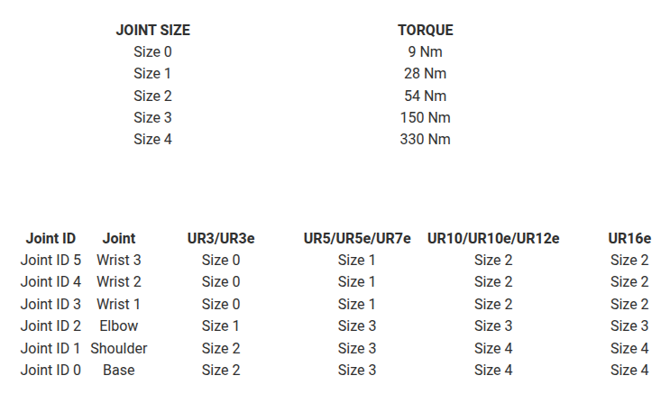
$$ \tau_{\textrm{sat}} \le \tau_{\max } $$
Use the figure below to construct the torque limit vector specific to your robot.
(If you simulate a different robot, make sure to update the torque limits)
Timing
You can control the frequency of your controller using the functions:
- r = rateControl(frequency)
- waitfor(r)
Other properties:
This controller needs to be fast. Try to achieve a frequency of 50 - 200 Hz for a stable simulation. If your hardware is not capable of this, you can reduce the simulation speed using the function:
- SetSimulationSpeed(Speedfactor) with Speedfactor \(\in \left(\left\lbrack 0,1\right\rbrack \right)\)
- or SetSimulationSpeed(Speedfactor, 'docker',false) for native Ubuntu
Optional Visualization:
You can store the joint states, speeds and torques and visualize them using the function:
- plotTrajectory(qstorage, qdstorage, tau_storage)
Start the Simulation by running:
%StartTutorialApplication('Simulation','Controller', 'Effort', 'Model','ur3e');
%If you use ROS on a native Ubuntu system use:
StartTutorialApplication('Simulation','Controller', 'Effort', 'Model','ur3e', 'Docker', false);
To see the path of the end effector you can run:
%StartTutorialApplication('Trajectory');
%If you use ROS on a native Ubuntu system use:
StartTutorialApplication('Trajectory', 'Docker', false);
StartTutorialApplication('Safety_nodes','docker',false); %sends a 0 torque when no other command has been sent
Load the Robot and setup the gravity vector
robot = [];
robot.Gravity = [];
Setup your Parameters here
tau_lim = [];
Kp = []
Kd = [];
q_desired = [];
qd_desired = [];
Setup your control loop
you can use tic and toc execute the while loop for a desired time.
check your hardware performance and see analyze your rate of publishing. To do this, increment a counter each loop execution and after the loop has finished divide by the elapsed time.
qstorage = [];
qdstorage = [];
tau_storage = [];
time = [];
Execution_time = 10;
count = 0;
t0 = tic;

while toc(t0)<Execution_time

end
Plot your trajectory
plotTrajectory(qstorage,qdstorage,tau_storage)
Try a different Model
Inspect the effects of an incorrect dynamics model by loading the ur3e robot into your MATLAB workspace while simulating an ur5e model.
StopTutorialApplications('docker',false);
clear SendJointTorques GetJointValues
StartTutorialApplication('Simulation','Controller', 'Effort', 'Model','ur5e', 'Docker', false);
StartTutorialApplication('Trajectory', 'Docker', false);
StartTutorialApplication('Safety_nodes','docker',false); %sends a 0 torque when no other command has been sent
tau_lim = [150 150 150 28 28 28]'; %UR5e
robot = importrobot(["robotics/Resources/urdf/ur3e.urdf"], DataFormat="column");
g = [0,0,-9.81]';
robot.Gravity=g;