clear all
Modelling with Robotic System Toolbox
This tutorial explains how to set up a robot in the Robotic System Toolbox.
General
The Robotic System Toolbox uses Structures to define the Robot manipulators.
You can create a rigidBodyTree to fill it with your robot values. Define the DataFormat as column or row for dynamic calculations.
robot = rigidBodyTree("DataFormat","column")
robot =
  rigidBodyTree with properties:

     NumBodies: 0
        Bodies: {1x0 cell}
          Base: [1x1 rigidBody]
     BodyNames: {1x0 cell}
      BaseName: 'base'
       Gravity: [0 0 0]
    DataFormat: 'column'
    FrameNames: {'base'}
We now need to fill this objects fields with the values corresponding to the robot.
Create a Robot
Let's consider a simple planar robot:

and its DH parameters:
| Link | a [m] | alpha | d [m] | theta |
| 1 | 0.30 | 0 | 0 | 0 |
| 2 | 0.25 | pi/2 | 0 | 0 |
        %a      alpha   d       theta
DH_1 = [0.3     0       0       0];
DH_2 = [0.25    pi/2    0       0];
additionally we have an translation and rotation from the base to the first joint. This can be represented by the following homogeneous transform matrix:
$$ T_{\textrm{B0}} =\left\lbrack \begin{array}{cccc} 0 & 1 & 0 & 0\newline -1 & 0 & 0 & -0\ldotp 1\newline 0 & 0 & 1 & 0\newline 0 & 0 & 0 & 1 \end{array}\right\rbrack $$
TB0= [  0,  1,  0,  0;
        -1, 0,  0,  -0.1;
        0,  0,  1,  0;
        0,  0,  0,  1 ];
first create empty body and joint cell arrays
bodies = cell(3,1);
joints = cell(3,1);
define the bodies as a rigidBody and assign a name to each body
bodies{1} = rigidBody('body_base');
bodies{2} = rigidBody('body_1');
bodies{3} = rigidBody('body_2');
define the joints as a rigidBodyJoint, set their name and define if it is a revolute, prismatic or fixed joint.
joints{1} = rigidBodyJoint('base_link', 'fixed');
joints{2} = rigidBodyJoint('joint_1', 'revolute');
joints{3} = rigidBodyJoint('joint_2', 'revolute');
If one a joint has a limit in terms of viable positions we can set the position limits. Lets consider the first revolute joint to be restricted by \(\theta {\;}_{\textrm{Joint}\;1} \in \left\lbrack 0\;,\pi \right\rbrack\)
joints{2}.PositionLimits = [0 , pi];
define the transforms for the joints. Add the parameter 'dh' to let the toolbox know you are feeding it data in DH format. You may also pass a homogeneous transform matrix.
For a revolute joint the system will automatically disregard the "theta" parameter, as theta is the joint action. For prismatic joints the "d" parameter will be disregarded as it is the joint action.
setFixedTransform(joints{1}, TB0);
setFixedTransform(joints{2}, DH_1, 'dh');
setFixedTransform(joints{3}, DH_2, 'dh');
add the joints to the bodies:
bodies{1}.Joint = joints{1};
bodies{2}.Joint = joints{2};
bodies{3}.Joint = joints{3};
finally, add the bodies to the robot structure.
The first body is connected to the base.
addBody(robot, bodies{1}, "base");
The following bodies are connected to their predecessor.
You can manually input their names:
addBody(robot, bodies{2}, 'body_base')
or access the previously defined names
addBody(robot, bodies{3}, bodies{2}.Name);
To access and change values from the robot joints after adding the bodies to the robot, we can use structure and cell notation. To change the joint limits we can:
robot.Bodies{2}.Joint.PositionLimits = [-pi,pi/2];
To add offsets for a joint state ("theta" for revolute or "d" for prismatic joints) you can define their home position. These values will be the default for showing the robot.
For this sample robot we will use the "theta" parameter stored at the 4th position of our DH parameters
robot.Bodies{2}.Joint.HomePosition = DH_1(4);
robot.Bodies{3}.Joint.HomePosition = DH_2(4);
additionally we need to set the direction and magnitude of gravity w.r.t. the base frame:
robot.Gravity = [0, 9.81, 0];
showdetails(robot)
--------------------
Robot: (3 bodies)

 Idx        Body Name       Joint Name       Joint Type        Parent Name(Idx)   Children Name(s)
 ---        ---------       ----------       ----------        ----------------   ----------------
   1        body_base        base_link            fixed                 base(0)   body_1(2)
   2           body_1          joint_1         revolute            body_base(1)   body_2(3)
   3           body_2          joint_2         revolute               body_1(2)
--------------------
Visualize the Robot Structure
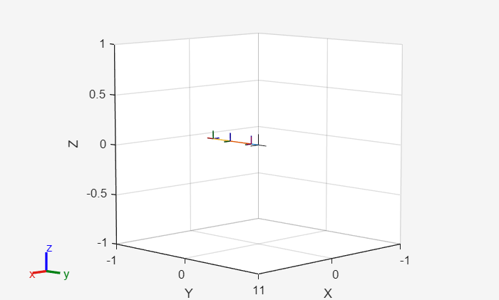
To view the robot in MATLAB you can use the show() function, it will show the robot in its home configuration:
show(robot)
ans =
  Axes (Primary) with properties:

             XLim: [-1 1]
             YLim: [-1 1]
           XScale: 'linear'
           YScale: 'linear'
    GridLineStyle: '-'
         Position: [0.1300 0.1100 0.7750 0.8150]
            Units: 'normalized'

  Show all properties
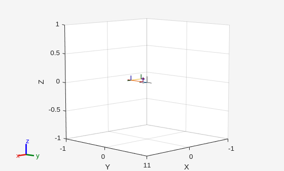
To view the robot in another configuration:
myconfig_2 = [0;-pi/2];  %column vector because we defined the robot as: robot = rigidBodyTree("DataFormat","column")
show(robot, myconfig_2) %we only have two joints
ans =
  Axes (Primary) with properties:

             XLim: [-1 1]
             YLim: [-1 1]
           XScale: 'linear'
           YScale: 'linear'
    GridLineStyle: '-'
         Position: [0.1300 0.1100 0.7750 0.8150]
            Units: 'normalized'

  Show all properties
Visualize in Rviz
In this tutorial can use the ROS2 visualization tool Rviz.
To start Rviz:
StartTutorialApplication('Rviz','model','ur3e');
ws_root = '/home/user'
wsPath = 'fctr_ws'
wsAbs = '/home/janrosell/fctr_ws'
FCTR-container
%StartTutorialApplication('Rviz','model','ur3e', 'docker',false); %use this
%when using a native ROS workspace
You can specify any UR model, e.g. 'ur5e' ( default is ur3e).
Once Rviz is running you can send it a desired configuration like:
myconfig = [0,-pi/2,0,-pi/2,0,0];
JointStatesToRviz(myconfig, 'ur3e');