Exercise 5.4 - Universal Robots in task space using velocity control

So far all control implementation have been made in joint space.

In this exercise you will setup a velocity controller operating in task space.

Load the Robot

Select a UR of your choice and load it either via the urdf files or from the robotic system toolbox.

urmodel = 'universalUR3e';
robot = loadrobot(robotmodel, DataFormat="column");

Start the Simulation

Don't forget to select the same robot as the model.

StartTutorialApplication('simulation','model', urmodel, 'controller','velocity', 'docker',false)
StartTutorialApplication('safety_nodes', 'docker',false)
StartTutorialApplication('trajectory','docker',false) %sends a 0 torque when no other command has been sent

Remember that you can slow down the simulation as:

SetSimulationSpeed( SpeedFactor, 'docker', false)

Joint Limits

Setup the velocity limit as:

$$ {\dot{\;q} }_{\lim } =\left\lbrack \begin{array}{c} 0\ldotp 7\newline 0\ldotp 7\newline 0\ldotp 7\newline 0\ldotp 7\newline 0\ldotp 7\newline 0\ldotp 7 \end{array}\right\rbrack \left\lbrack \frac{\textrm{rad}}{s}\right\rbrack $$

Goal Configurations

Try different configuration and convert it into a homogeneous transform matrix. Use configurations that do not result in a singularity.

Store them as:

T_desired_1
T_desired_2
T_desired_3

Using joint configurations and the forward kinematics ensures the resulting transforms are reachable by the robot.

$$ T_{\textrm{desired},i} \left(q_{\textrm{config},i} \right)=\textrm{forward}\textrm{kinematics}\left(q{\textrm{config},i} \right) $$

or using the Robotic System Toolbox function as

$T_{\textrm{desired},i}$ = getTransform(robot, config_i, "tool0", "base_link");

However you can also try other transform matrices. You can build them by using the transl() and trotm(angle, 'axis') functions.

visualize the configurations in rviz:

Published static transform: base_link → target_1
Published static transform: base_link → target_2
Published static transform: base_link → target_3

Singular Configurations

Below we will setup some singular configurations.

singular_configuration1 = [0,-pi/2,0,-pi/2,0,0]'; 
Singular_1 = getTransform(robot, singular_configuration1, "tool0", "base_link");
StaticFrameBroadcaster(Singular_1, 'singular_1');

Published static transform: base_link → singular_1

singular_configuration2 = [pi/3,0,0,-pi/2,0,0]'; 
Singular_2 = getTransform(robot, singular_configuration2, "tool0", "base_link");
StaticFrameBroadcaster(Singular_2, 'singular_2');

Published static transform: base_link → singular_2

Error computation

This controller operates in task space, meaning that errors are computed directly from the desired and current homogeneous transformation matrices.

Let

$$ T_{\textrm{desired}} =\left\lbrack \begin{array}{cc} R_{\textrm{desired}} & t_{\textrm{desired}} \newline 0 & 1 \end{array}\right\rbrack $$

$$ T_{\textrm{current}} \left(q\right)=\left\lbrack \begin{array}{cc} R_{\textrm{current}} & t_{\textrm{current}} \newline 0 & 1 \end{array}\right\rbrack $$

with the rotation matrix $R_i \in \mathbb{R}{\;}^{3\textrm{x3}} \;$ and the position vector $t_i \in {\mathbb{R}}^{3\textrm{x1}}$

Position Error (task space)

the position error computation is straight forward:

$$ e_{\textrm{pos}} =t_{\textrm{desired}} -t_{\textrm{current}} $$

Orientation Error (task space)

The orientation error is not as straightforward.

Euler angle representations are unsuitable because they suffer from gimbal lock and discontinuities.

To compute a singularity-free orientation error, the rotation matrices are first converted to unit quaternions.

The error quaternion is computed as a quaternion product:

$$ q_{\textrm{error}} =q_{\textrm{desired}} \otimes q_{\textrm{current}}^{-1} $$

Note that the operand $\otimes$ is not a normal multiplication.

Quaternions

Remember a unit quaternion is made up of 4 values:

$$ q=\left\lbrack \begin{array}{c} w\newline v \end{array}\right\rbrack =\left\lbrack \begin{array}{c} w\newline x\newline y\newline z \end{array}\right\rbrack $$

where

w is the scalar part
v the vector part
and $||q||=1$

The conjugate of a quaternion can be build as:

$$ q^{-1} =\left\lbrack \begin{array}{c} w\newline -v \end{array}\right\rbrack $$

Quaternion Error

Compute the orientation error as follows.

let

$q_{\textrm{desired}} =\left\lbrack \begin{array}{c} w_d \newline v_d \end{array}\right\rbrack$ and $q_{\textrm{current}}^{-1} =\left\lbrack \begin{array}{c} w_{\textrm{current}} \newline -v_{\textrm{current}} \end{array}\right\rbrack =\left\lbrack \begin{array}{c} w_c \newline v_c \end{array}\right\rbrack$

compute the error quaternion as:

$$ q_{\textrm{error}} =\left\lbrack \begin{array}{c} w_e \newline v_e \end{array}\right\rbrack $$

with

$$ w_e =w_d \cdot w_c -v_d^T \cdot v_c $$

and

$$ v_e =w_d \cdot v_c +w_c \cdot v_d +v_d \times v_c $$

(The operand $\times$ is a cross product)

A quaternion q and -q represent the same orientation.

To ensure that we use the shortest rotation to align the orientations, you must set the error quaternion as:

$ $ \left\lbrace \begin{array}{ll} q_e =\left\lbrack \begin{array}{c} w_e \newline v_e \end{array}\right\rbrack & \textrm{if}\;w_e >0\ q_e =\left\lbrack \begin{array}{c} -w_e \newline -v_e \end{array}\right\rbrack & \textrm{if}\;w_e <0 \end{array}\right. $ $

Compute error vector $e_{\textrm{ori}}$

let

$$ \textrm{nv}=||v_e || $$

then you can compute the angle $\theta$ as:

$$ \theta =2\cdot \textrm{atan2}\left(\textrm{nv},w_e \right) $$

finally compute $e_{\textrm{ori}}$ depending on the angle as:

$ $ \left\lbrace \begin{array}{ll} e_{\textrm{ori}} =\left\lbrack \begin{array}{c} 0\newline 0\newline 0 \end{array}\right\rbrack & \textrm{if}\;\theta <{10}^{-10} \ e_{\textrm{ori}} =\theta \cdot \frac{v_e }{||v_e ||}=\theta \cdot \frac{v_e }{\textrm{nv}} & \textrm{if}\;\theta >{10}^{-10} \end{array}\right. $ $

Weighted Error

As the manipulability of the position is generally smaller than the manipulability of the orientation, we have to apply a weights to the error to account for this.

Initialize with these weights and update them if you have to:

$ K_{\textrm{position}} = $ $ \left\lbrack \begin{array}{ccc} 1 & 0 & 0\newline 0 & 1 & 0\newline 0 & 0 & 1 \end{array}\right\rbrack $

$ K_{\textrm{orientation}} = $ $ \left\lbrack \begin{array}{ccc} 0\ldotp 5 & 0 & 0\newline 0 & 0\ldotp 5 & 0\newline 0 & 0 & 0\ldotp 5 \end{array}\right\rbrack $

$$ e_{\textrm{position}} =K_{\textrm{position}} \cdot e_{\textrm{pos}} $$

$$ e_{\textrm{orientation}} =K_{\textrm{orientation}} \cdot e_{\textrm{ori}} $$

Initialize your weights here

build the error with respect to your jacobian:

$ $ e=\left\lbrace \begin{array}{ll} \left\lbrack \begin{array}{c} e_{\textrm{position}} \newline e_{\textrm{orientation}} \end{array}\right\rbrack & \textrm{if}\;J=\left\lbrack \begin{array}{c} J_p \newline J_{\theta \;} \end{array}\right\rbrack \;\ \left\lbrack \begin{array}{c} e_{\textrm{orientation}} \newline e_{\textrm{position}} \end{array}\right\rbrack & \textrm{if}\;J=\left\lbrack \begin{array}{c} J_{\theta \;} \newline J_p \end{array}\right\rbrack \; \end{array}\right. $ $

Pseudoinverse Jacobian with least square damping

We can improve the behavior of the robot near singularities by using a least square damping jacobian pseudo inverse.

Compute it as follows:

$$ J_{\lambda \;}^{\dagger} =J^T \cdot {\left({J\cdot \;J}^T +2\cdot \lambda^2 \cdot I\right)}^{-1} $$

Dashboard

Once you open the simulink file, you'll see a dashboard with multiple input and monitoring options.

Transform selector

Allows you to switch between your previously defined transformations.

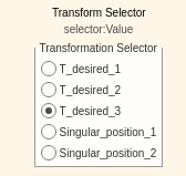
selecting a transform will switch the input from:

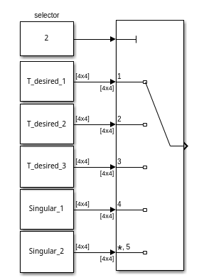
make sure all Transformations are loaded in your workspace.

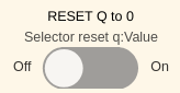
Reset configuration

Some required joint velocities may result in your robot joints reaching their limits ( $\pm 2\pi$ for all joints except the last wrist joint). You can flip the switch while in simulation to move all joints to 0.

Lambda selection

you can tune your lambda during simulation by using the slider.

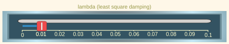
The slider value can be used in the constant block:

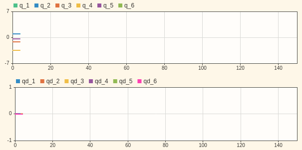
Monitoring States

You have two live plots showing your the joint configuration q and the joint velocities qd.

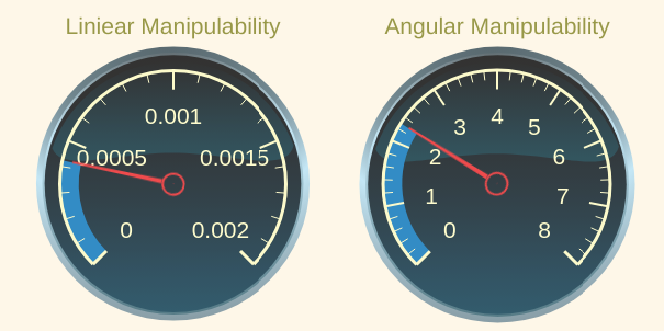
Monitoring Manipulability

You have two gauges showing you the current manipulability index. Their limits are setup for a UR3e model.

If you use a larger model, you may have to adjust the limits.

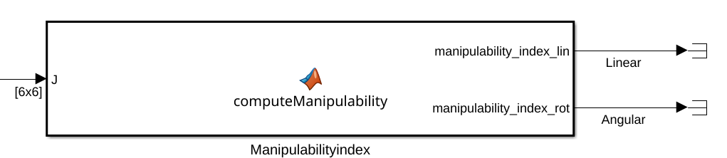
The measurements are linked to the output of this matlab function block:

Simulink Blocks

You can solve this exercise by using the following (new) Simulink Blocks.

Get Jacobian (Robotic System Toolbox)

select:

'robot' as the robot
'tool0' as the End Effector.

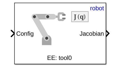
Inputs:

Input a joint configuration obtained from the GetJointValues subsystem as $q\in \mathbb{R}{\;}^{6\textrm{x1}}$

Outputs:

The Jacobian as $J\left(q\right)=\left\lbrack \begin{array}{c} J_{\theta \;} \newline J_p \end{array}\right\rbrack$

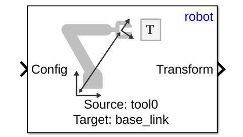
Get Transform (Robotic System Toolbox)

specify:

'robot' as Ridged body tree
'tool0' as the Source body
'base_link' as the Target body

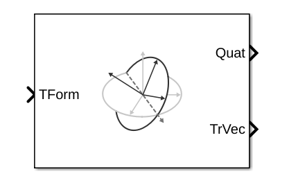
Coordinate Transformation Conversion (Robotic System Toolbox)