clear all
Modelado con Robotic System Toolbox
Este tutorial explica cómo configurar un robot en la Robotic System Toolbox.
General
La Robotic System Toolbox usa estructuras para definir los manipuladores robóticos.
Puedes crear un rigidBodyTree para rellenarlo con los valores de tu robot. Define DataFormat como column o row para cálculos dinámicos.
robot = rigidBodyTree("DataFormat","column")
robot =
  rigidBodyTree with properties:

     NumBodies: 0
        Bodies: {1x0 cell}
          Base: [1x1 rigidBody]
     BodyNames: {1x0 cell}
      BaseName: 'base'
       Gravity: [0 0 0]
    DataFormat: 'column'
    FrameNames: {'base'}
Ahora necesitamos rellenar los campos de este objeto con los valores correspondientes al robot.
Crear un robot
Consideremos un robot planar simple:

y sus parámetros DH:
| Eslabón | a \(begin:math:display\)m\(end:math:display\) | alpha | d \(begin:math:display\)m\(end:math:display\) | theta |
| 1 | 0.30 | 0 | 0 | 0 |
| 2 | 0.25 | pi/2 | 0 | 0 |
        %a      alpha   d       theta
DH_1 = [0.3     0       0       0];
DH_2 = [0.25    pi/2    0       0];
además tenemos una traslación y rotación desde la base hasta la primera articulación. Esto puede representarse mediante la siguiente matriz de transformación homogénea:
$$ T_{\textrm{B0}} =\left\lbrack \begin{array}{cccc} 0 & 1 & 0 & 0\newline -1 & 0 & 0 & -0\ldotp 1\newline 0 & 0 & 1 & 0\newline 0 & 0 & 0 & 1 \end{array}\right\rbrack $$
TB0= [  0,  1,  0,  0;
        -1, 0,  0,  -0.1;
        0,  0,  1,  0;
        0,  0,  0,  1 ];
primero crea arrays de celdas vacíos para cuerpos y articulaciones
bodies = cell(3,1);
joints = cell(3,1);
define los cuerpos como rigidBody y asigna un nombre a cada cuerpo
bodies{1} = rigidBody('body_base');
bodies{2} = rigidBody('body_1');
bodies{3} = rigidBody('body_2');
define las articulaciones como rigidBodyJoint, establece su nombre y define si es una articulación rotativa, prismática o fija.
joints{1} = rigidBodyJoint('base_link', 'fixed');
joints{2} = rigidBodyJoint('joint_1', 'revolute');
joints{3} = rigidBodyJoint('joint_2', 'revolute');
Si una articulación tiene un límite en términos de posiciones viables, podemos establecer los límites de posición. Consideremos que la primera articulación rotativa está restringida por \(\theta {\;}_{\textrm{Joint}\;1} \in \left\lbrack 0\;,\pi \right\rbrack\)
joints{2}.PositionLimits = [0 , pi];
define las transformaciones para las articulaciones. Añade el parámetro 'dh' para que la toolbox sepa que le estás proporcionando datos en formato DH. También puedes pasar una matriz de transformación homogénea.
Para una articulación rotativa, el sistema ignorará automáticamente el parámetro "theta", ya que theta es la acción articular. Para articulaciones prismáticas, el parámetro "d" se ignorará, ya que es la acción articular.
setFixedTransform(joints{1}, TB0);
setFixedTransform(joints{2}, DH_1, 'dh');
setFixedTransform(joints{3}, DH_2, 'dh');
añade las articulaciones a los cuerpos:
bodies{1}.Joint = joints{1};
bodies{2}.Joint = joints{2};
bodies{3}.Joint = joints{3};
finalmente, añade los cuerpos a la estructura del robot.
El primer cuerpo está conectado a la base.
addBody(robot, bodies{1}, "base");
Los cuerpos siguientes están conectados a su predecesor.
Puedes introducir manualmente sus nombres:
addBody(robot, bodies{2}, 'body_base')
o acceder a los nombres definidos previamente
addBody(robot, bodies{3}, bodies{2}.Name);
Para acceder a valores de las articulaciones del robot y cambiarlos después de añadir los cuerpos al robot, podemos usar notación de estructuras y celdas. Para cambiar los límites articulares podemos hacer:
robot.Bodies{2}.Joint.PositionLimits = [-pi,pi/2];
Para añadir offsets a un estado articular ("theta" para articulaciones rotativas o "d" para prismáticas), puedes definir su posición inicial. Estos valores serán los predeterminados al mostrar el robot.
Para este robot de ejemplo usaremos el parámetro "theta" almacenado en la 4.ª posición de nuestros parámetros DH
robot.Bodies{2}.Joint.HomePosition = DH_1(4);
robot.Bodies{3}.Joint.HomePosition = DH_2(4);
además necesitamos establecer la dirección y magnitud de la gravedad respecto al sistema de la base:
robot.Gravity = [0, 9.81, 0];
showdetails(robot)
--------------------
Robot: (3 bodies)

 Idx        Body Name       Joint Name       Joint Type        Parent Name(Idx)   Children Name(s)
 ---        ---------       ----------       ----------        ----------------   ----------------
   1        body_base        base_link            fixed                 base(0)   body_1(2)
   2           body_1          joint_1         revolute            body_base(1)   body_2(3)
   3           body_2          joint_2         revolute               body_1(2)
--------------------
Visualizar la estructura del robot
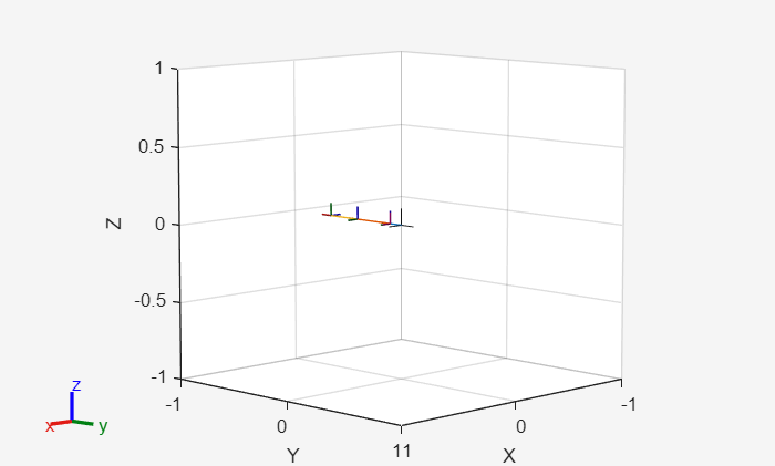
Para ver el robot en MATLAB puedes usar la función show(), que mostrará el robot en su configuración inicial:
show(robot)
ans =
  Axes (Primary) with properties:

             XLim: [-1 1]
             YLim: [-1 1]
           XScale: 'linear'
           YScale: 'linear'
    GridLineStyle: '-'
         Position: [0.1300 0.1100 0.7750 0.8150]
            Units: 'normalized'

  Show all properties
Para ver el robot en otra configuración:
myconfig_2 = [0;-pi/2];  %vector columna porque hemos definido el robot como: robot = rigidBodyTree("DataFormat","column")
show(robot, myconfig_2) %solo tenemos dos articulaciones

%Esta configuración es la necesaria para JointStatesToRviz
myconfig = [0,-pi/2,0,-pi/2,0,0];
Visualizar en Rviz
En este tutorial puedes usar la herramienta de visualización de ROS2 Rviz.
Para arrancar Rviz:
StartTutorialApplication('Rviz','model','ur3e');
%StartTutorialApplication('Rviz','model','ur3e', 'docker',false); %use this
%when using a native ROS workspace
Puedes especificar cualquier modelo UR, por ejemplo 'UR5e' (el modelo por defecto es UR3e).
Una vez que Rviz esté ejecutándose, puedes enviarle una configuración deseada como:
myconfig = [0,-pi/2,0,-pi/2,0,0];
JointStatesToRviz(myconfig, 'ur5e');