clear all;
Exercise 3.1 - Jacobian
In this exercise you will setup different functions relating to the jacobian of a UR3e robot.
Consider this UR3e robot and its dimensions.
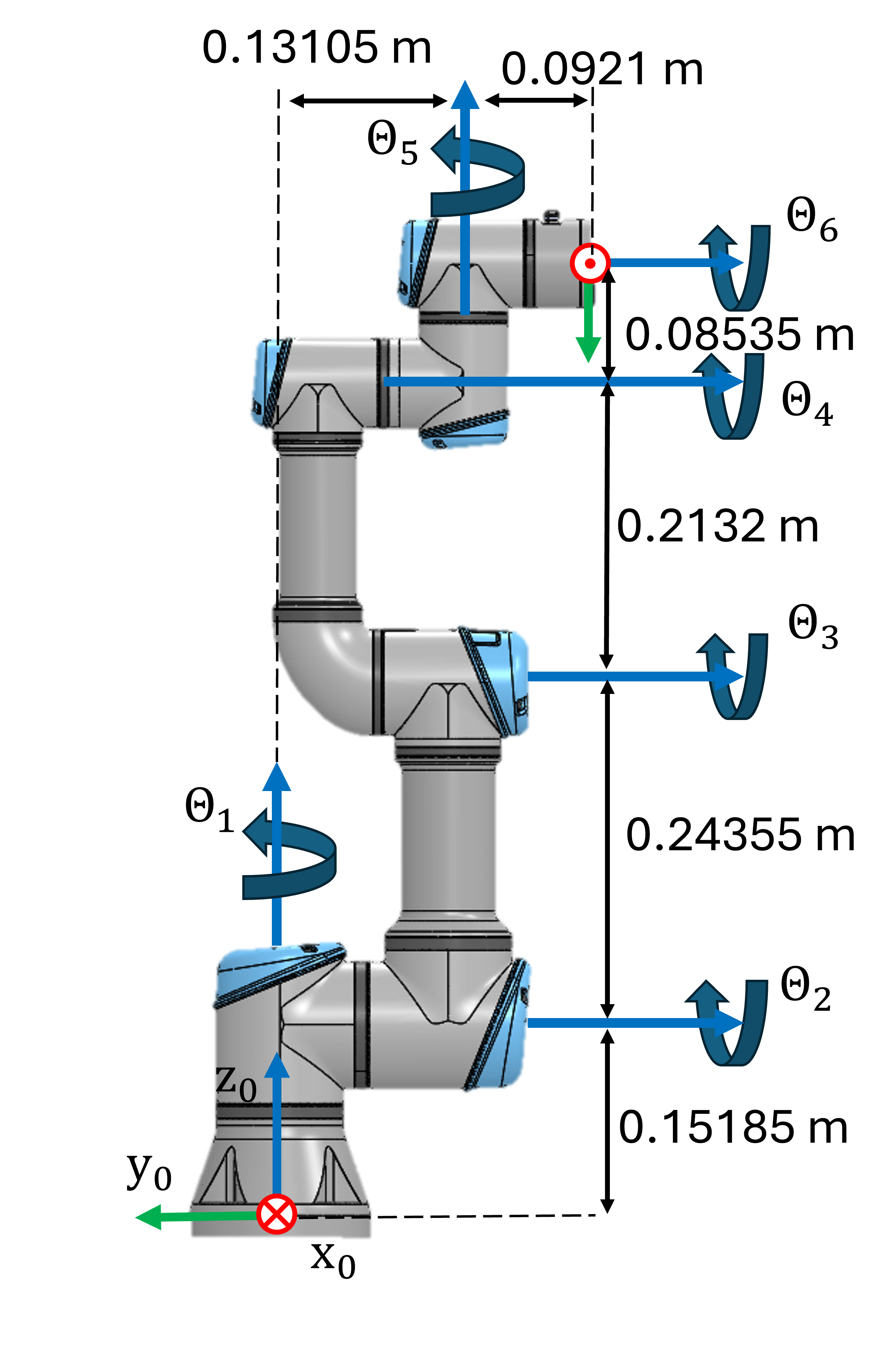
Task 1
Setup the geometric Jacobian using the symbolic toolbox. The resulting symbolic expression should only depend on the joint states
- Find the DH parameters and setup the Jacobian matrix.
Use the following variables to store your solution:
- q1 ... q6 (Real Symbolic variable for the Joint angle Theta 1-6)
- Jp (translational part of the Jacobian)
- Jtheta (rotational part of the Jacobian)
- J (complete Jacobian as \(J\left(q\right)=\left\lbrack \begin{array}{c} J_{\theta } \left(q\right)\newline J_p \left(q\right) \end{array}\right\rbrack\) )
Solve this exercise using the geometric approach! Use the function:
- cross()
Solve this exercise without using the function:
- dh2tf()
and without using the relation matrix \(T_A \left(\Phi \right)\):
- \(\displaystyle T_A \left(\Phi \right)=\left\lbrack \begin{array}{ccc} 0 & -\sin \left(\phi \right) & \cos \left(\phi \right)\cdot \sin \left(\theta \right)\newline 0 & -\sin \left(\phi \right)\cdot \sin \left(\theta \right) & -\sin \left(\phi \right)\cdot \sin \left(\theta \right)\newline 1 & \cos \left(\theta \right) & \cos \left(\theta \right) \end{array}\right\rbrack\)
Jp = [];
Jtheta = [];
J = [];
You can check your work by clicking the Run:
check_exercise('3-1-1')
Task 2
Write a function that computes the analytical jacobian (using ZYZ euler angles) for a given configuration. This function takes one vector as an input:
- Configures (q) as a row vector ( \(q\in {\mathbb{R}}^{6\textrm{x1}}\) )
and returns the analytical jacobian as \(J_a \left(q\right)=\left\lbrack \begin{array}{c} J_{\Phi \;} \left(q\right)\newline J_p \left(q\right) \end{array}\right\rbrack\) and its rank at the configuration.
Use the following function name for your solution:
- ComputeAnalyticalJacobian(q)
Solve this exercise using an analytical approach! Use the function:
- diff()
Solve this exercise without using the relation matrix \(T_A \left(\Phi \right)\):
- \(\displaystyle T_A \left(\Phi \right)=\left\lbrack \begin{array}{ccc} 0 & -\sin \left(\phi \right) & \cos \left(\phi \right)\cdot \sin \left(\theta \right)\newline 0 & -\sin \left(\phi \right)\cdot \sin \left(\theta \right) & -\sin \left(\phi \right)\cdot \sin \left(\theta \right)\newline 1 & \cos \left(\theta \right) & \cos \left(\theta \right) \end{array}\right\rbrack\)
function [Ja, Rank] = ComputeAnalyticalJacobian(q)
Ja = 6x6
1.0000    0.0000    0.0000    0.0000    1.0000         0
         0   -0.0000   -0.0000   -0.0000    0.0000         0
         0    1.0000    1.0000    1.0000    0.0000    1.0000
    0.2231   -0.5421   -0.2985   -0.0853    0.0921         0
    0.0000         0         0         0    0.0000         0
         0    0.0000    0.0000    0.0000   -0.0000         0

Rank = 4
Ja = [];
Rank = rank(Ja);

end
You can check your work by clicking the Run:
check_exercise('3-1-2')
Error using fileread (line 10)
Could not open file exercises\exercise-3-1-2.json. No such file or directory.

Error in check_exercise (line 8)
    data = jsondecode( fileread(json_file) );
    ^^^^^^^^^^^^^^^^^^^^^^^^^^^^^^^^^^^^^^^^^
Task 3
Write a function that computes the required joint velocities to achieve a specific translational motion of the endeffector for a given configuration. Only consider the endeffector position and not its orientation. This function takes two vectors as an input:
- configuration (q) as a row vector ( \(q\in {\mathbb{R}}^{6\textrm{x1}}\) )
- desired motion v, relative to the base frame, as a row vector where \(v=\left\lbrack \begin{array}{c} \dot{x} \newline \dot{y} \newline \dot{z} \end{array}\right\rbrack\)
and returns the required joint speeds as a row vector ( \(\dot{q} \in {\mathbb{R}}^{6\textrm{x1}}\) ) and the rank of the Jacobian.
Use the following function name for your solution:
- ComputeJointSpeed(q,v)
Solve this exercise using a geometric approach! Use the function:
- cross()
function [qdot , Rank]= ComputeJointSpeed(q,v)

qdot = [];
Rank = [];

end
You can check your work by clicking the Run:
check_exercise('3-1-3')
Task 4
Use your function from Task 3 to compute a trajectory that follows the desired motion.
Approximate the new joint states by \(q_{k+1} =q_k +\dot{q} \cdot \Delta t\) where \(\dot{q}\) is the computed joint velocity for the configuration \(q_k\).
The function takes four inputs:
- Initial Joint configuration (q)
- desired motion (v)
- timestep (dt)
- total time (T)
The function has three outputs:
- Joint State trajectory ( \(q_{\textrm{traj}} \in {\mathbb{R}}^{6\textrm{xN}}\) where N is the amount of points in the trajectory, usually \(N=\frac{T}{\Delta t}\) )
- Joint Velocity trajectory ( \(\dot{q_{\textrm{traj}} } \in {\mathbb{R}}^{6\textrm{xN}}\) )
- Success, false if the manipulator hits a singularity in the desired motion dimensions (success \(\in \left\lbrack \textrm{false},\textrm{true}\right\rbrack\) ). If a singularity is reached the function needs to end and send the joint states until the singularity
Use the following function name for your solution:
- ComputeLinearTrajectory(q, v, dt, T)
function [q_traj, qdot_traj, success] = ComputeLinearTrajectory(q,v, dt, T)

end
You can check your work by clicking the Run:
check_exercise('3-1-4')
You can view your trajectory in Rviz:
q_example = [-2.5408, -1.3607, 0.7146, 0.3767, 1.7134, 0]';
v_example = [-0.5;-0.5;0];
dt_example =0.01;
T_example = 1;
[q_traj_ex, q_dot_traj ,success_example] = ComputeLinearTrajectory(q_example, v_example, dt_example, T_example);

if success_example
    JointStatesToRviz(q_traj_ex, 'ur3e', T_example);
else
    [~,points_until_singular,~] = size(q_traj_ex);
    Time_until_singular = points_until_singular*dt;
    JointStatesToRviz(q_traj_ex, 'ur3e', Time_until_singular, 'Ellipsoid', true);
end

plotTrajectory(q_traj_ex, q_dot_traj, linspace(0,T_example,T_example/dt_example))
Try adjusting some parameters and see how the trajectory behaves. Keep in mind that the computation may take some time depending on the resolution and hardware.