Exercise 5.2 - Threelink effort control using PD control and extenstions
In this exercise you will use a PD to control scheme the Threelink manipulator in simulation using Simulink.
Start the Simulation
StartTutorialApplication('Simulation','Controller', 'Effort', 'Model','threelink', 'Docker', false);
StartTutorialApplication('Trajectory', 'Docker', false);
StartTutorialApplication('Safety_nodes','docker',false, 'model','threelink'); %sends a 0 torque when no other command has been sent
Remember that you can slow down the simulation as:
SetSimulationSpeed( SpeedFactor, 'docker', false)
Parameters
Setup the tau limit as:
$$ {\textrm{tau}}_{\lim } =\left\lbrack \begin{array}{c} 120\newline 120\newline 60 \end{array}\right\rbrack \left\lbrack \textrm{Nm}\right\rbrack $$
and the desired configuration (both speed and position)
try the configurations
$$ q\in \left\lbrace \left\lbrack \begin{array}{c} -\frac{\pi }{3}\newline \frac{\pi }{3}\newline \frac{\pi }{10} \end{array}\right\rbrack ,\left\lbrack \begin{array}{c} -\pi \;\newline \frac{\pi }{5}\newline \frac{\pi }{6}\; \end{array}\right\rbrack ,\left\lbrack \begin{array}{c} \frac{\pi }{8}\newline -\frac{\textrm{pi}}{2}\newline \frac{\textrm{pi}}{3} \end{array}\right\rbrack \right\rbrace $$
store them as:
- q_desired_1
- q_desired_2
- q_desired_3
- qd_desired
taulim = [120,120,60]';
q_desired_1 = [-pi/3, pi/3, pi/10]';
q_desired_2 = [-pi,pi/5,pi/6]';
q_desired_3 = [pi/8,-pi/2,pi/3]';
qd_desired = [0,0,0]';
to visualize the target transforms in Rviz:
load("5.Control/Resources/targetTransform_threelink.mat");
StaticFrameBroadcaster(targetTransform_threelink_1, 'target1');
Published static transform: base_link → target1
StaticFrameBroadcaster(targetTransform_threelink_2, 'target2');
Published static transform: base_link → target2
StaticFrameBroadcaster(targetTransform_threelink_3, 'target3');
Published static transform: base_link → target3
To try any other configuration you can:
syms q1 q2 q3 real
DH =    [3/10, pi/2, 1/5, q1;
         1/2,    0,   0,  q2;
         1/2,    0,   0,  q3];
T03 = dh2tf(DH);

q_desired_3 = [pi/8,-pi/2,pi/3]'; % insert your configuration here
targetTransform = double(subs(T03, [q1,q2,q3], q_desired_3'));
StaticFrameBroadcaster(targetTransform, 'target3');
Published static transform: base_link → Target_frame
Task 1 PD Control scheme
Task 1.1 - Gain Selection
The PD control scheme does not cancel the non linearities as the inverse dynamic control scheme from Exercise 4.2 and 5.1. While the inverse dynamic scheme scales the selected gains with the inertia matrix, this is not the case here.
To have a starting point for your gain tuning, use the gains computed in Exercise 4.2 and scale them in the following way:
estimate the maximum values of the diagonal terms of the Inertia matrix B.
To estimate it without using an optimization algorithm, substitute all sin/cos functions with \(\pm 1\) so that the resulting value will be maximized.
Example:
$$ f\left(x_1 ,x_2 \right)=5\cdot \sin \left(x_1 \right)-2\cdot \cos \left(x_2 \right)+5\cdot \sin \left(\frac{x_1 }{x_2 }\right) $$
$$ \max \;\hat{\;f} \left(x_1 ,x_2 \right)=5\cdot 1-2\cdot -1+5\cdot 1=12 $$
Then multiply your previous gains with this estimation as:
$$ {\textrm{Kp}}{\textrm{PD}} =\max \hat{\;B} \left(q_1 ,q_2 ,q_3 \right)*{\textrm{Kp}}{\textrm{inverseDynamic}} $$
and
$$ {\textrm{Kd}}{\textrm{PD}} =\max \hat{\;B} \left(q_1 ,q_2 ,q_3 \right)*{\textrm{Kd}}{\textrm{inverseDynamic}} $$
(you will be able to scale the gains during simulation)
Use the symbolic Inertia matrix from Exercise 4.1 to compute your gains here:
w_i = 1x3
    3.8095    4.9689    7.1429
Dashboard
In the Simulink file you will find the dashboard section that allows you to switch between the configurations, see the current torque output and scale the Kp and Kd matrix during simulation.
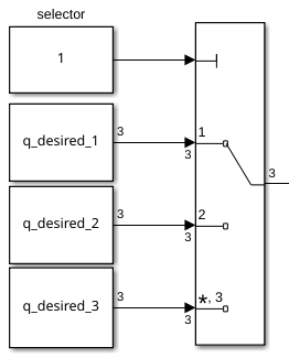
Configuration Selector
Check one of these boxes to select the desired configuration.
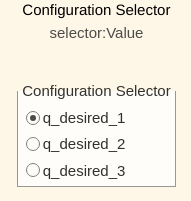
this selection block is linked to:
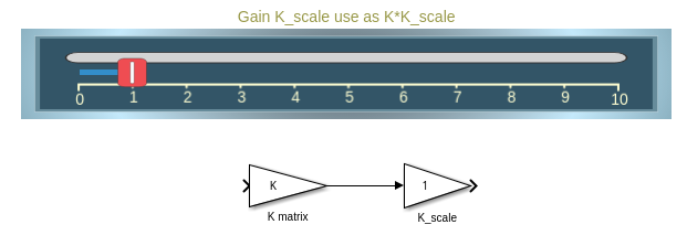
Scale Kd and Kp
By using the sliders you can alter the gain value of their corresponding K_scale blocks:
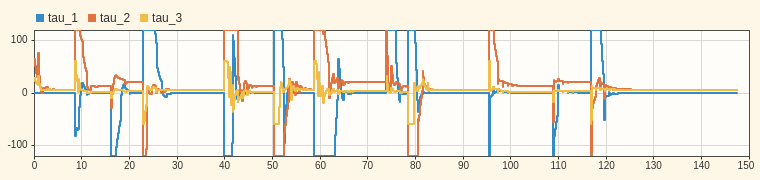
View Torque Trajectory
The Dashboard scope allows you to see the current torques live during simulation (like a scope).
Task 1.2
Setup a PD control scheme. Open the file Exercise_5_2_1.slx and setup the plant.
Analyze the behavior and see if the manipulator reaches its configuration.
you can load the simulation results into matlab with:
q_data_1 = out.position;
qd_data_1 = out.velocity;
tau_data_1 = out.tau;
t_data_1 = out.tout;
Plot your results in matlab.
Task 2 PD + Gravity Compensation
To reduce the steady state error we can improve the model by introducing the gravity compensation.
Task 2.1 Gravity term
convert your symbolic gravity matrix from Exercise 4.1 into a function as you did in Exercise 5.1 (or use the existing file).
Task 2.2 Update the plant
Open the file Exercise_5_2_2.slx and insert your plant from Task 1. Now add a MatlabFunction block and use the gravity matrix function.
The resulting control scheme should be (before applying saturation)
$$ \textrm{tau}={\textrm{Kp}}{\textrm{PD}} \cdot e+{\textrm{Kd}}{\textrm{PD}} \cdot \dot{\;e} +G\left(q\right) $$
Analyze the behavior of this improved control scheme.
Task 3 Integral Term
This scheme works well when you only care about the empty manipulator or the weight of the payload is neglectable. If this is not the case we can improve the behavior by introducing an integration term that grows whenever the robot is close to the configuration.
Integrator Gain Ki
Start by defining the Ki gain as:
$$ K_i =\left\lbrack \begin{array}{ccc} 1 & 0 & 0\newline 0 & 1 & 0\newline 0 & 0 & 1 \end{array}\right\rbrack $$
You can then scale it during simulation using the designated slider on the dashboard.
Anti Windup
It is important that the integral error term does not grow when the displacement is very large. One way of implementing an anti windup logic is using a matlab function block.
Write a function that takes the joint velocities and the position error as an input and output an integral error increment vector.
The output error vector should only contain non zero values in indices that have low joint velocity (The joints have reached their torque based on the non integral terms). Other values should be 0.
Integrator Block
Use the discrete-time integrator block.
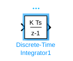
Select:
- 'Integration: Trapezoidal' as the Integrator method
- Set Gain value to 1.0
- 'either' as External reset
You have to reset the Integrator block when changing the reference configuration.
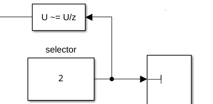
You can use a Detect Change block:
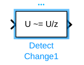
as an input you can use the Selector block from from the joint configuration selector. Thus whenever you change the goal configuration, you reset the integral.
Add a payload
You can add a payload to the endeffector by flipping the switch to Attach.
You can define the weight of the payload in grams.
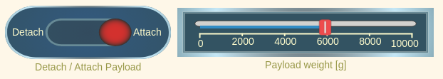
To attach a new payload first detach the old one, change the weight and attach it again.
When attaching a payload, make sure your endeffector is not moving, otherwise the payload may have an offset (not visible in Rviz).
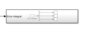
Visualize the error integral
Connect your integral error to the subsystem Error integral to view it on the dashboard