Exercise 5.1 - Threelink effort control using Symbolic Matrices
In this exercise you will use the matrices computed in Exercise 4.1 to control the Threelink manipulator in simulation using Simulink.
Start the Simulation
StartTutorialApplication('Simulation','Controller', 'Effort', 'Model','threelink', 'Docker', false);
StartTutorialApplication('Trajectory', 'Docker', false);
StartTutorialApplication('Safety_nodes','docker',false, 'model','threelink'); %sends a 0 torque when no other command has been sent
Remember that you can slow down the simulation as:
SetSimulationSpeed( SpeedFactor, 'docker', false)
Convert Symbolic Matrices to Functions
To use symbolic variables inside Simulink we have to convert them to a function.
syms symbolic1 symbolic2 real
my_sym_variable = [symbolic1^-1, symbolic2*4];
my_sym_vec = [symbolic1, symbolic2]
$$ \displaystyle \left(\begin{array}{cc} {\textrm{symbolic}}_1 & {\textrm{symbolic}}_2 \end{array}\right) $$
matlabFunction(my_sym_variable, 'vars',{my_sym_vec}, 'File','my_test_subs_function');
To use this function:
test_configuration = [2,2]
test_configuration = 1x2
     2     2
my_sym_variable_subsituted = my_test_subs_function(test_configuration)
my_sym_variable_subsituted = 1x2
    0.5000    8.0000
hint: This can be done using the MatlabFunction block in Simulink
Convert your Symbolic Matrices here
Unrecognized function or variable 'B'.
Parameters
Setup the tau limit as:
$$ {\textrm{tau}}_{\lim } =\left\lbrack \begin{array}{c} 120\newline 120\newline 60 \end{array}\right\rbrack \left\lbrack \textrm{Nm}\right\rbrack $$
and the desired configuration (both speed and position)
try the configurations
$$ q\in \left\lbrace \left\lbrack \begin{array}{c} -\frac{\pi }{3}\newline \frac{\pi }{3}\newline \frac{\pi }{10} \end{array}\right\rbrack ,\left\lbrack \begin{array}{c} -\pi \;\newline \frac{\pi }{5}\newline \frac{\pi }{6}\; \end{array}\right\rbrack ,\left\lbrack \begin{array}{c} \frac{\pi }{8}\newline -\frac{\textrm{pi}}{2}\newline \frac{\textrm{pi}}{3} \end{array}\right\rbrack \right\rbrace $$
store them as:
- q_desired_1
- q_desired_2
- q_desired_3
- qd_desired
taulim = [120,120,60]';
q_desired_1 = [-pi/3, pi/3, pi/10]';
q_desired_2 = [-pi,pi/5,pi/6]';
q_desired_3 = [pi/8,-pi/2,pi/3]';
qd_desired = [0,0,0]';
to visualize the target transforms in Rviz:
load("5.Control/Resources/targetTransform_threelink.mat");
StaticFrameBroadcaster(targetTransform_threelink_1, 'target1');
Published static transform: base_link → target1
StaticFrameBroadcaster(targetTransform_threelink_2, 'target2');
Published static transform: base_link → target2
StaticFrameBroadcaster(targetTransform_threelink_3, 'target3');
Published static transform: base_link → target3
Gains
Select the gains for your system, as this is an inverse dynamic scheme, follow the approach from Exercise 4.2. Don't scale the gains yet, you will be able to do so during simulation.
w_i = 1x3
    3.8095    4.9689    7.1429
Dashboard
In the Simulink file you will find the dashboard section that allows you to switch between the configurations, see the current torque output and scale the Kp and Kd matrix during simulation.
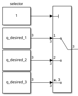
Configuration Selector
Check one of these boxes to select the desired configuration.
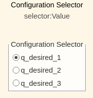
this selection block is linked to:
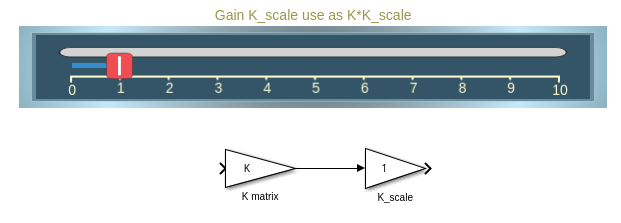
Scale Kd and Kp
By using the sliders you can alter the gain value of their corresponding K_scale blocks:
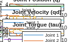
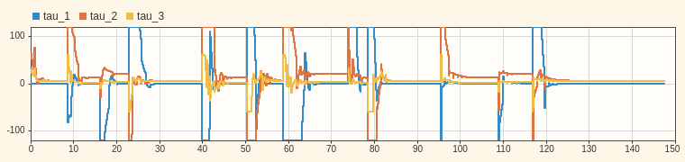
View Torque Trajectory
The Dashboard scope allows you to see the current torques live during simulation (like a scope).
Task 1
Open the File Exercise_5_1_1.slx you will find a setup to be used for this exercise. From the outputs q and qd (left Subsystem) you will receive the current position and velocity of the joints as a column vector.
The input to the right subsystem accepts a column vector and sends the torques to the simulation.
To import the results of your simulation into matlab:
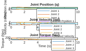
q_data_1 = out.position;
qd_data_1 = out.velocity;
tau_data_1 = out.tau;
t_data_1 = out.tout;
Plot your results in matlab.
Task 2
Reduce the computational load by only considering the diagonal terms of the B and C matrix and analyze the behavior and compare them to the results of Task 1.
Task 2.1
Setup the new symbolic matrix and convert them to a function.
Task 2.2
Open the File Exercise 5_1_2.slx and setup the plant with the new matrices B' and C'.
To import the results of your simulation into matlab: