Tutorial and exercises

This practical starts from a basic idea: a digital image can be understood as a matrix of pixels. Each pixel has a position in the image and contains visual information, either one gray-level value or several values associated with color. For this reason, concepts such as spatial resolution, quantization and the color model are important before applying any image-processing technique.

Throughout the tutorial, the operations are simple, but each one has a clear conceptual meaning. Some operations modify only pixel values, while others change the size, position or apparent shape of the image. Understanding this difference helps connect this first practical with later topics such as filtering, segmentation and object description.

Basic image manipulation

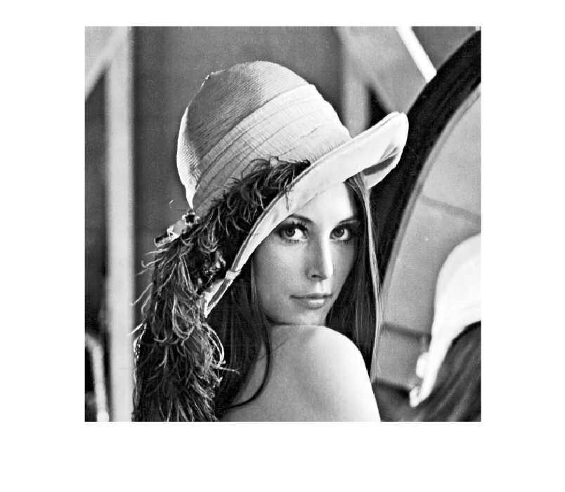
We load the images

I = imread("Imagenes\lena_gray_512.tif");
F = imread("Imagenes\lena_color_512.tif");

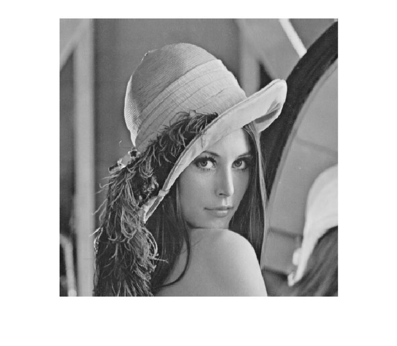
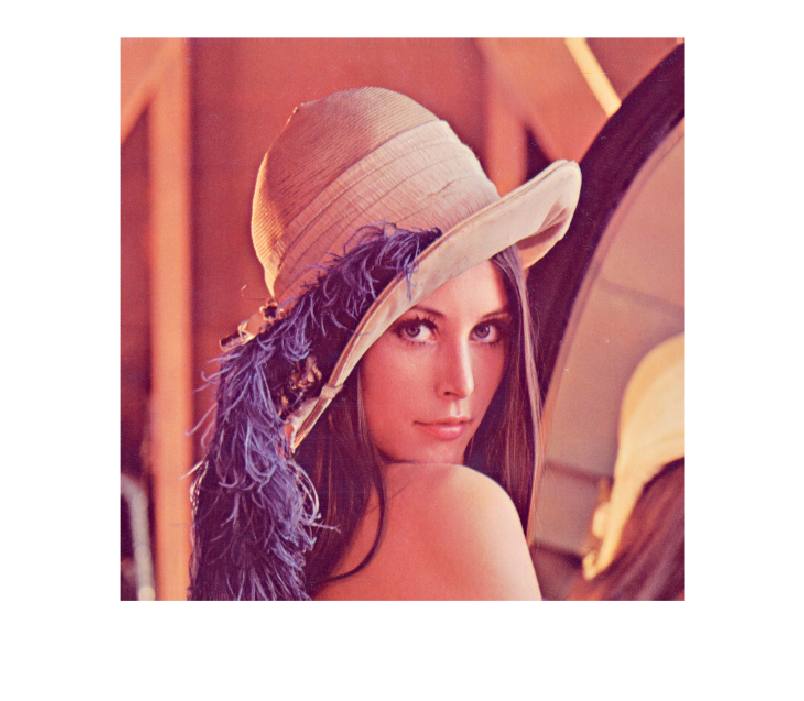
We display the images

imshow(I)

imshow(F)

We calculate the spatial resolution of each image

Spatial resolution indicates the number of pixels that form the image in width and height. A higher resolution can represent more detail if the original capture contains that detail, but resizing an already digitized image does not add real information. When an image is enlarged or reduced, new values must be estimated from existing pixels, and this may smooth details or create artifacts.

size(I)

ans = 1x2
   512   512

size(F)

ans = 1x3
   512   512     3

We calculate the intensity resolution, or quantization, of each image

Intensity resolution, also called quantization, indicates how many different levels each pixel can represent. In an 8-bit image there are 256 possible values, from 0 to 255. If this number of levels is reduced, different scene intensities are represented by the same value, which may cause loss of fine contrast or visible banding in smooth regions.

max(max(I))

ans = uint8245

max(max(F))

ans = 1x1x3 uint8 array
ans(:,:,1) =

   255

ans(:,:,2) =

   248

ans(:,:,3) =

   225

We spatially rescale the image

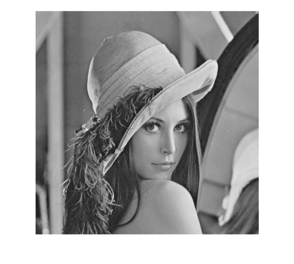
Spatial rescaling means changing the number of pixels in the image. If the image is reduced, samples are removed and detail may be lost. If the image is enlarged, intermediate values must be estimated by interpolation; therefore, enlargement does not recover real detail that was not present in the original image.

I = imresize(I,[128,128]);
imshow(I)

I = imresize(I,[64,64]);
imshow(I)

I = imresize(I,[16,16]);
imshow(I)

I = imread("Imagenes\lena_gray_512.tif");
I = imresize(I,[1028,1028]);
imshow(I)

We rescale the intensity levels of the image

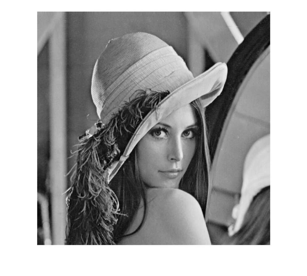
Rescaling intensity levels means changing the range of pixel values. This operation can make an image look brighter, darker or higher contrast, but it does not change the position of objects. It is useful for preparing images before applying thresholds or filters.

levels_gray = [128,32,4];

I_128 = imquantize(I, linspace(0, 255, levels_gray(1)));
I_32 = imquantize(I, linspace(0, 255, levels_gray(2)));
I_4 = imquantize(I, linspace(0, 255, levels_gray(3)));

imshow(I_128,[])

imshow(I_32,[])

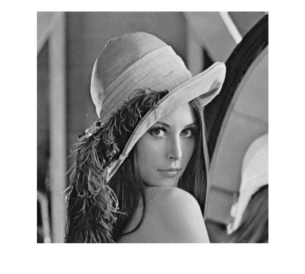
imshow(I_4,[])

We calculate the histogram

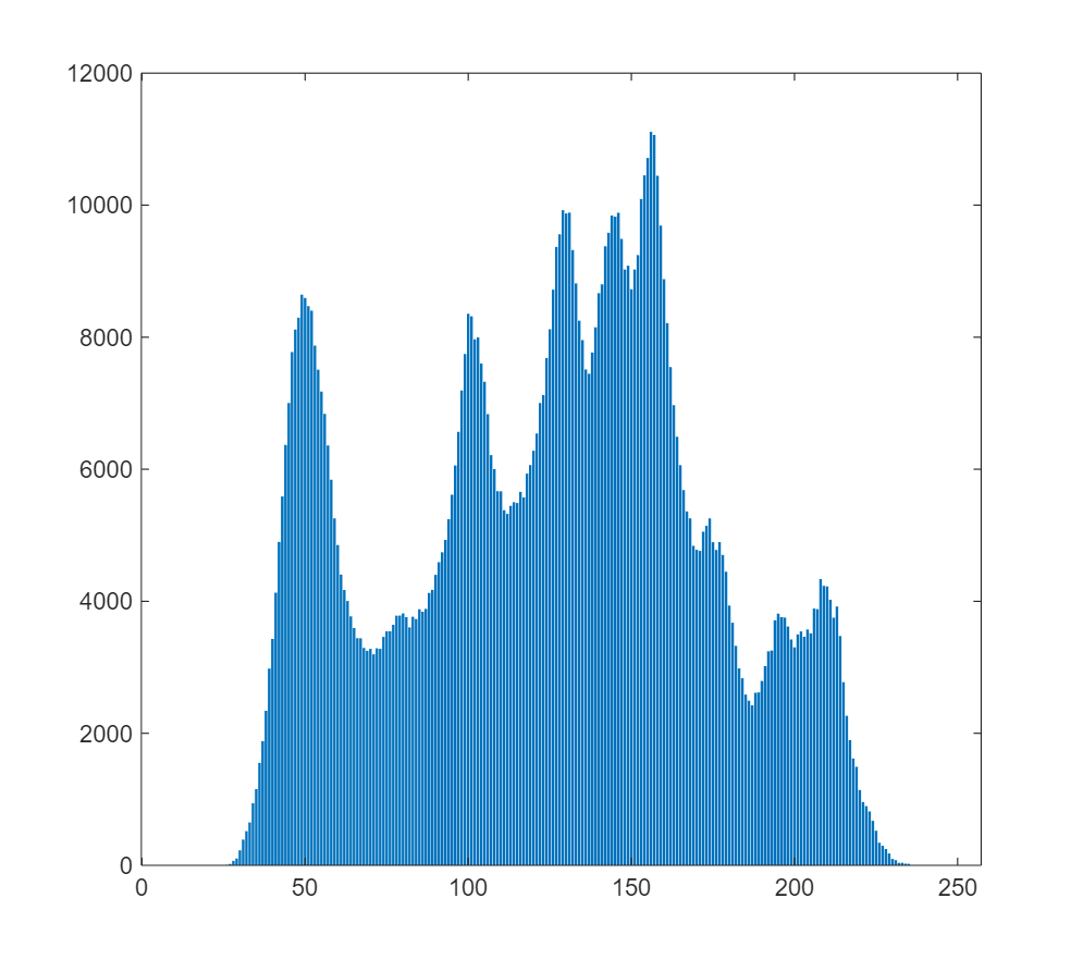
The histogram is a simple tool for studying the distribution of intensity levels in an image. It shows how many pixels have each value, but it does not preserve information about their position. Even with this limitation, it is very useful for detecting whether an image is dark, bright, low contrast, or whether it contains groups of intensities that could be separated with a threshold.

histograma = imhist(I);

We visualize the histogram

bar(histograma)

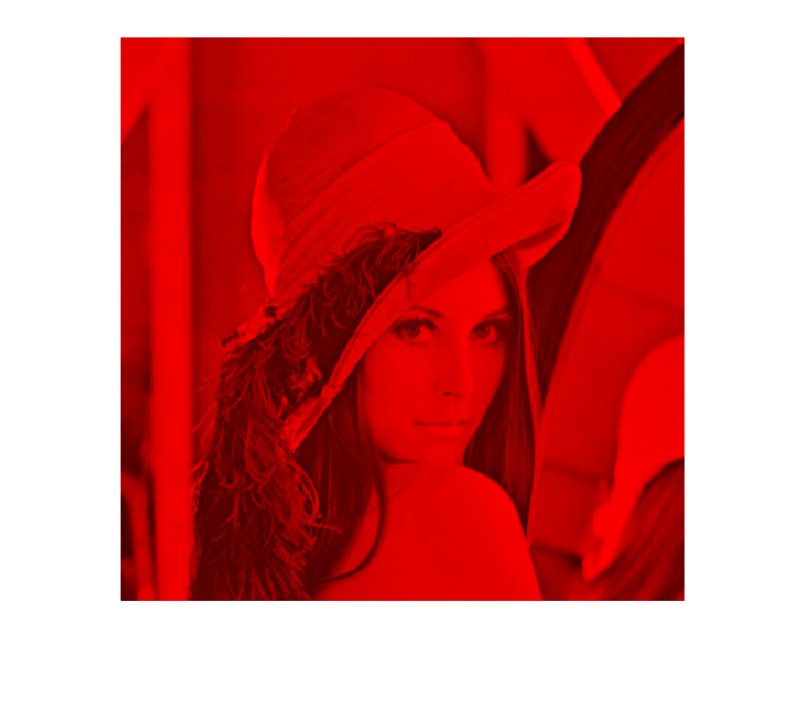
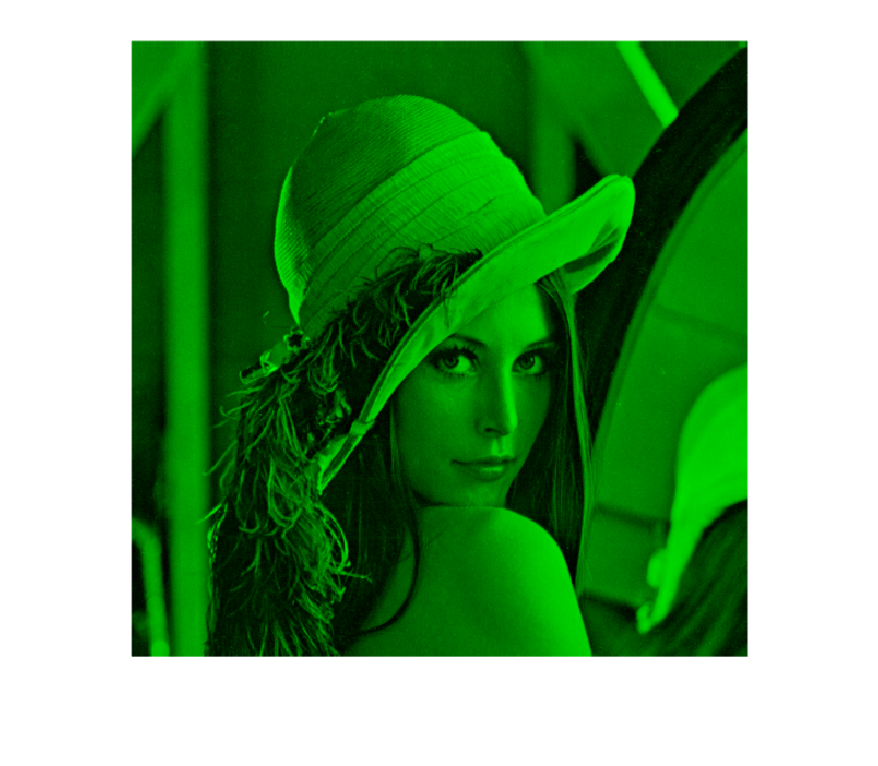
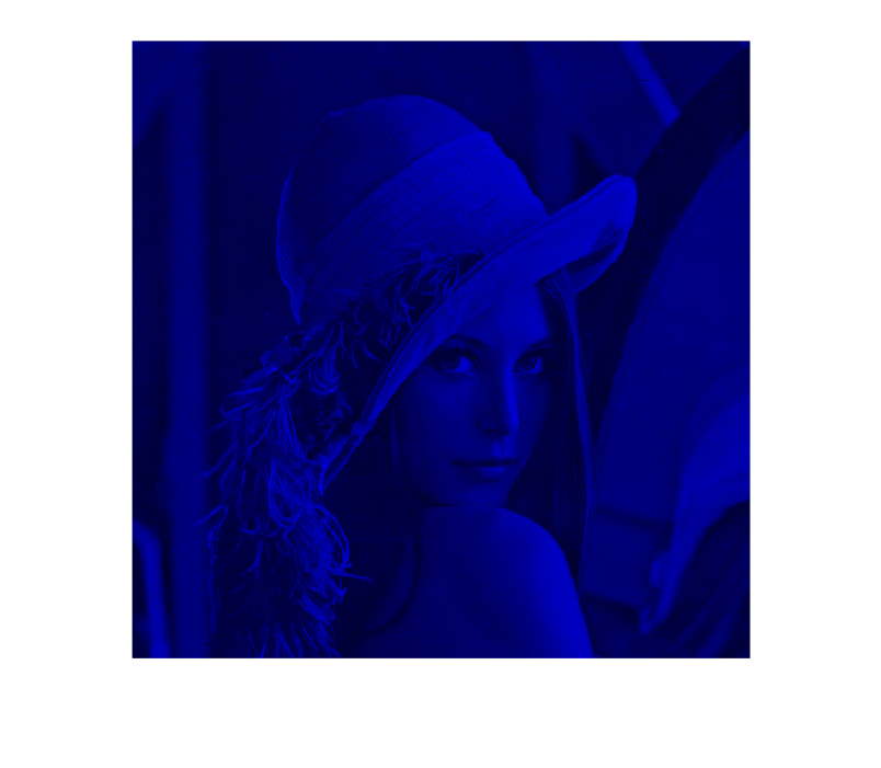
We calculate each of the color channels of the image by "removing" the other two

Separating color channels helps show that the color of a pixel is a combination of several components. In the RGB model, each channel represents the contribution of red, green or blue. In the HSV model, color is described using hue, saturation and perceived intensity, which can be more suitable for some visual-analysis tasks.

F_rojo = F;
F_rojo(:,:,2)=0;
F_rojo(:,:,3)=0;

F_verde = F;
F_verde(:,:,1)=0;
F_verde(:,:,3)=0;

F_azul = F;
F_azul(:,:,1)=0;
F_azul(:,:,2)=0;

imshow(F_rojo)

imshow(F_verde)

imshow(F_azul)

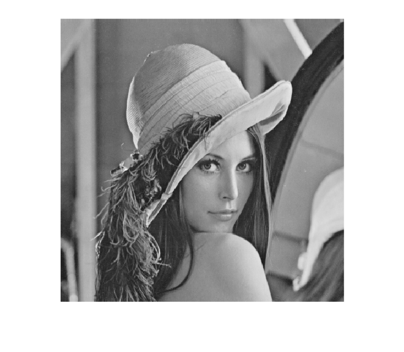
We convert the image from RGB to grayscale

Converting to grayscale reduces a three-channel image to a single intensity image. This is usually not a simple average of the channels, but a weighted combination that takes visual sensitivity to red, green and blue into account. Color information is lost, but analysis is simpler when color is not essential.

F_gris = rgb2gray(F);
imshow(F_gris)

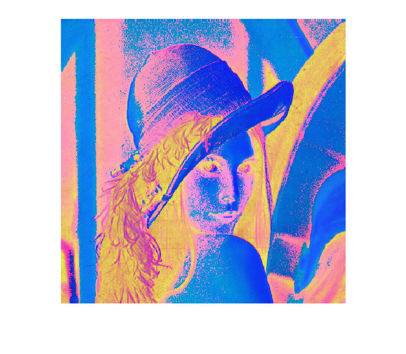
We convert the image from RGB to HSV

The HSV model separates color information into three more interpretable components: hue indicates the type of color, saturation indicates color purity, and value indicates brightness. This separation can help in tasks where color should be analyzed more independently from illumination.

F_hsi = rgb2hsv(F);
imshow(F_hsi)

We calculate the H, S and V channels

imshow(F_hsi(:,:,1))

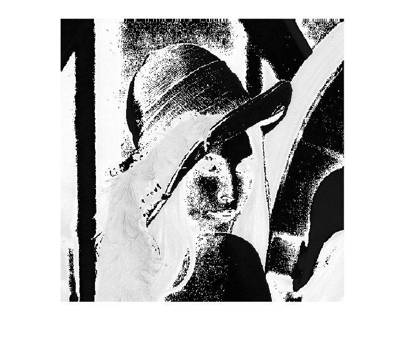
imshow(F_hsi(:,:,2))

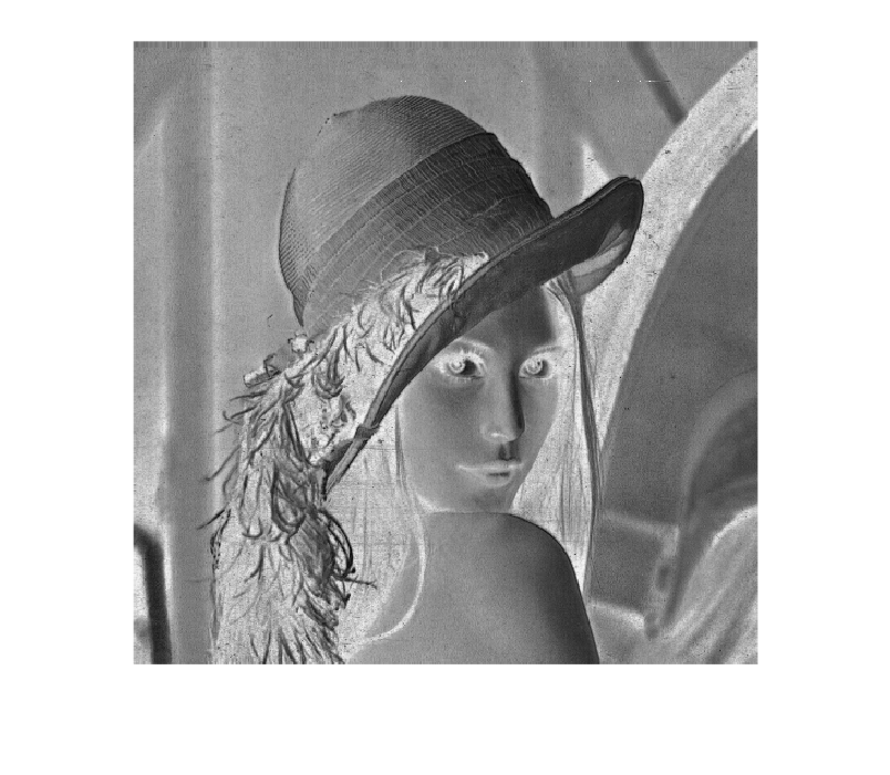
imshow(F_hsi(:,:,3))

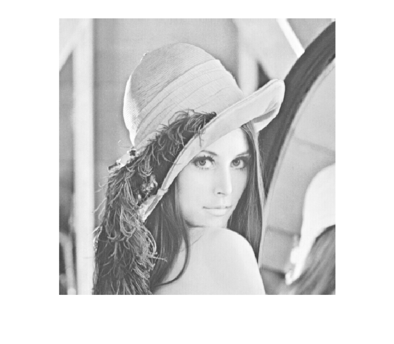
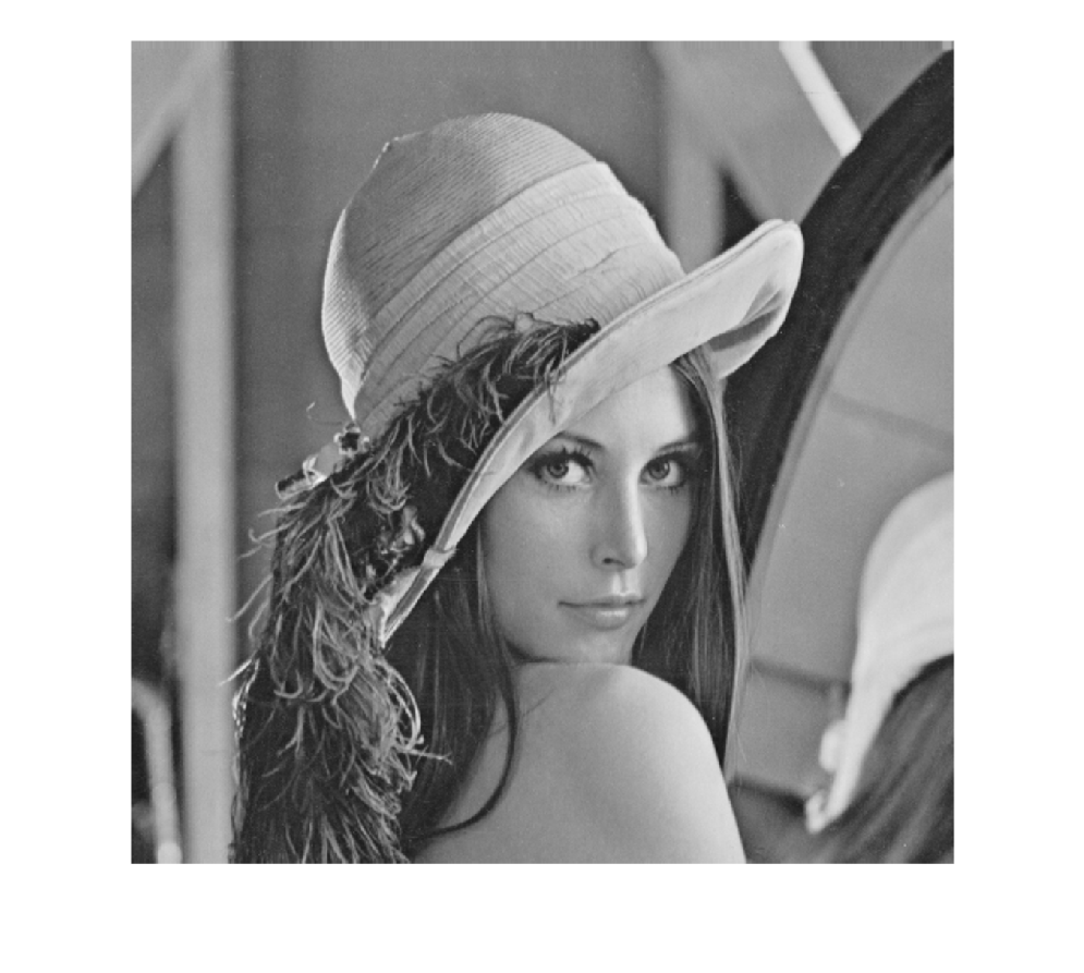
Gaussian noise

Noise represents unwanted changes in pixel values. It may appear because of limitations in the sensor, illumination, transmission or digitization process. In Gaussian noise, many pixels undergo small changes around an average value, so the image keeps its general structure but obtains a more grainy appearance.

We define the Gaussian noise parameters, that is, the mean and variance

media = 0;
varianza = 0.01;

The imnoise function adds multiplicative Gaussian noise, which can be easily detected by its grainy appearance

In multiplicative noise, the perturbation depends on the pixel value. This means that brighter regions may be affected differently from darker regions. This model is useful for understanding noise that is not added equally across the whole image.

I_gaussian_mult = imnoise(I,"gaussian",media,varianza);

imshow(I_gaussian_mult)

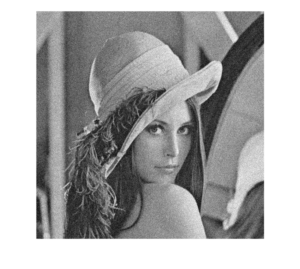
Whereas additive Gaussian noise, which is added directly to the image, only slightly blurs the details

In additive noise, each pixel receives a random variation that is independent of its original value. The image keeps its general structure, but small local differences may be contaminated. This is why many smoothing filters try to reduce this type of local variation.

ruido_gaussiano = uint8(randn(size(I)) * sqrt(varianza) + media);

I_gaussian_add = I + ruido_gaussiano;

imshow(I_gaussian_add)

Salt and pepper noise

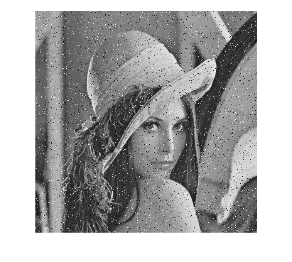
Salt-and-pepper noise is an example of impulsive noise. Unlike Gaussian noise, it does not affect all pixels smoothly, but replaces some values with extreme intensities, usually black or white. This behavior explains why, in later practicals, nonlinear filters such as the median can be more appropriate than a simple average.

We define the parameters of salt and pepper noise, namely, the probability that a given pixel becomes a salt or pepper grain

probabilidad = 0.05;

Generate a random image that we use to change the pixels of the original image to salt or pepper points (if a random pixel is above or below the defined probability, the corresponding pixel in the original image is changed)

ruido_sal_pimienta = rand(size(I));
I_ruido = I;

I_ruido(ruido_sal_pimienta < probabilidad/2) = 0; % "salt" noise
I_ruido(ruido_sal_pimienta > 1 - probabilidad/2) = 255; % "pepper" noise

imshow(I_ruido)

Arithmetic operations

Arithmetic operations act directly on the numerical values of pixels. Adding or subtracting can modify brightness, while multiplying or dividing can change global contrast. It is important to remember that digital images have a limited value range; if an operation produces values outside that range, information may be lost because of saturation.

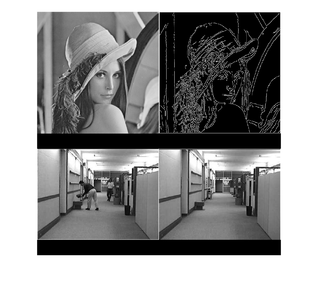
I = imread("Imagenes\lena_gray_512.tif");

F = imread("Imagenes\Contornos.tif");

G = imread("Imagenes\Office1.png");

H = imread("Imagenes\Office2.png");

G = rgb2gray(G);

H = rgb2gray(H);

montage({I,F,G,H})

Arithmetic addition by a constant

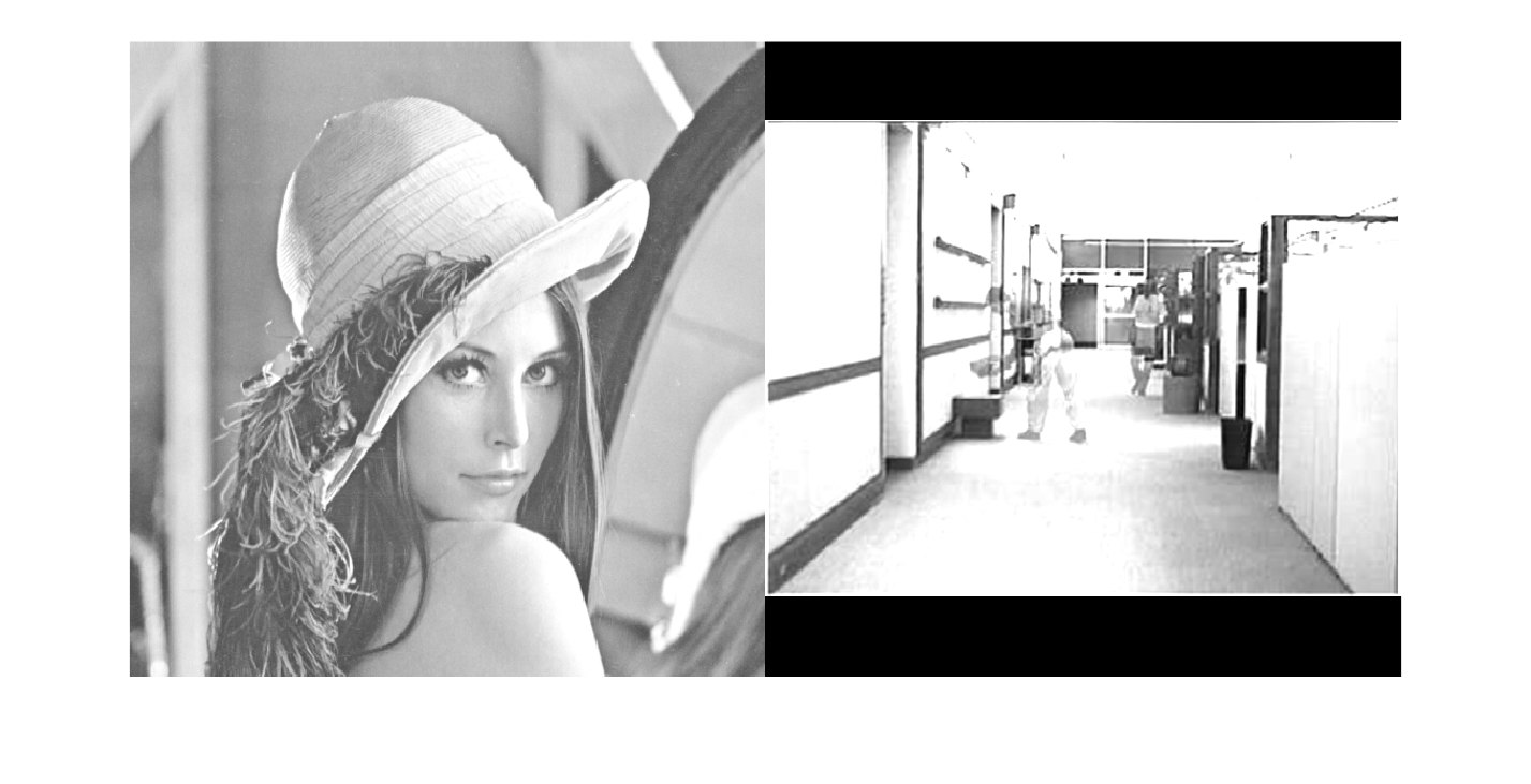
I_50 = I + 50;

We rescale so that we can operate with the images and use the add function to add them

s = size(G);

H = imresize(H,[s(1),s(2)]);

GH_add = imadd(G,H);

montage({I_50,GH_add})

Subtraction by a constant

I_75 = I - 75;

We rescale so that we can operate with the images and use the subtract function to subtract them

F = rgb2gray(imresize(F,[512,512]));

IF_resta = imsubtract(I,F);

montage({I_75,IF_resta})

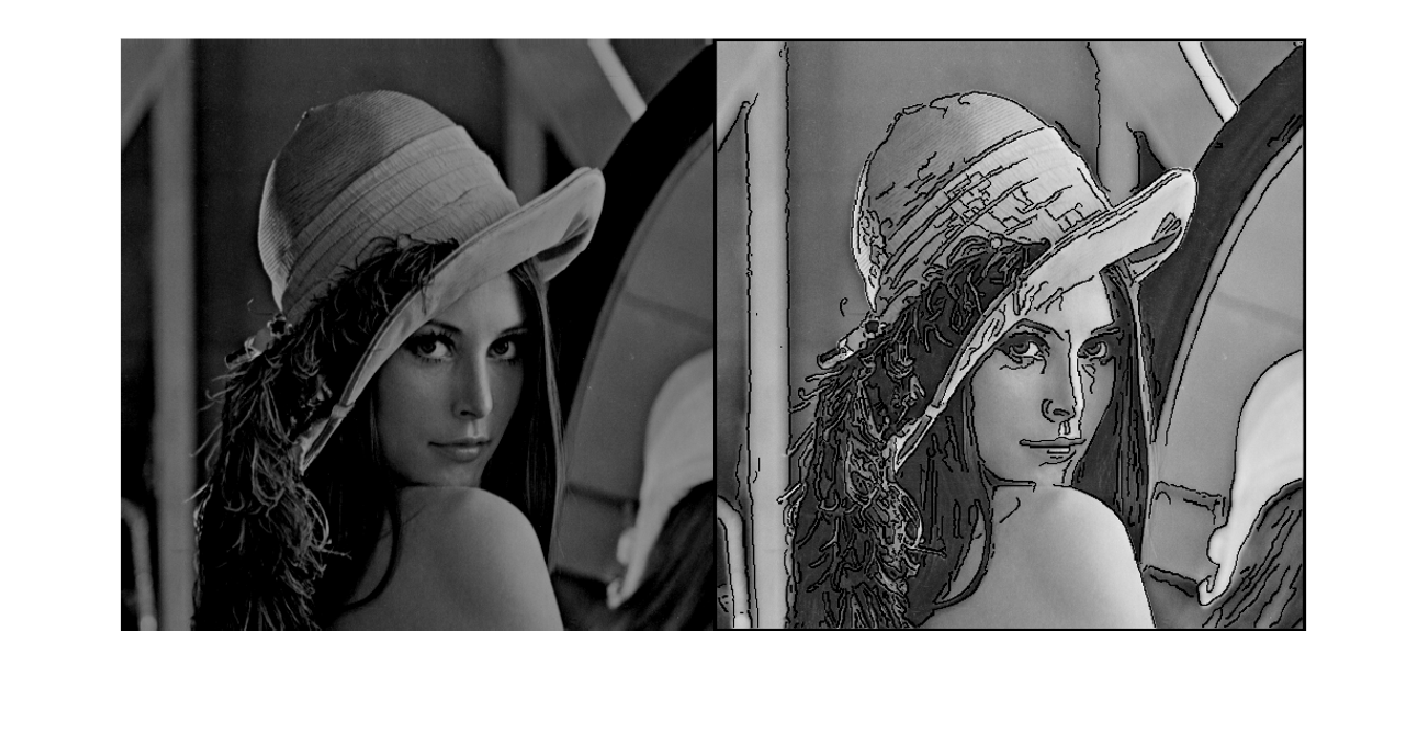
Product by a constant

I_2 = I.*2;

We rescale so that we can operate with the images and use the immultiply function to multiply them

IG_prod = immultiply(I,imresize(G,[512,512]));

montage({I_2,IG_prod})

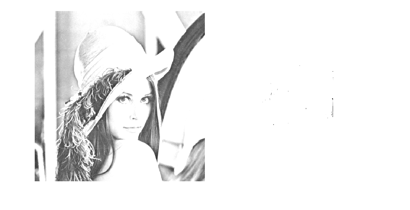
Division by a constant

I__2 = I./2;

We rescale so that we can operate with the images and use the imdivide function to divide them

I_div = imdivide(I,imresize(G,[512,512]));

montage({I__2,I_div})

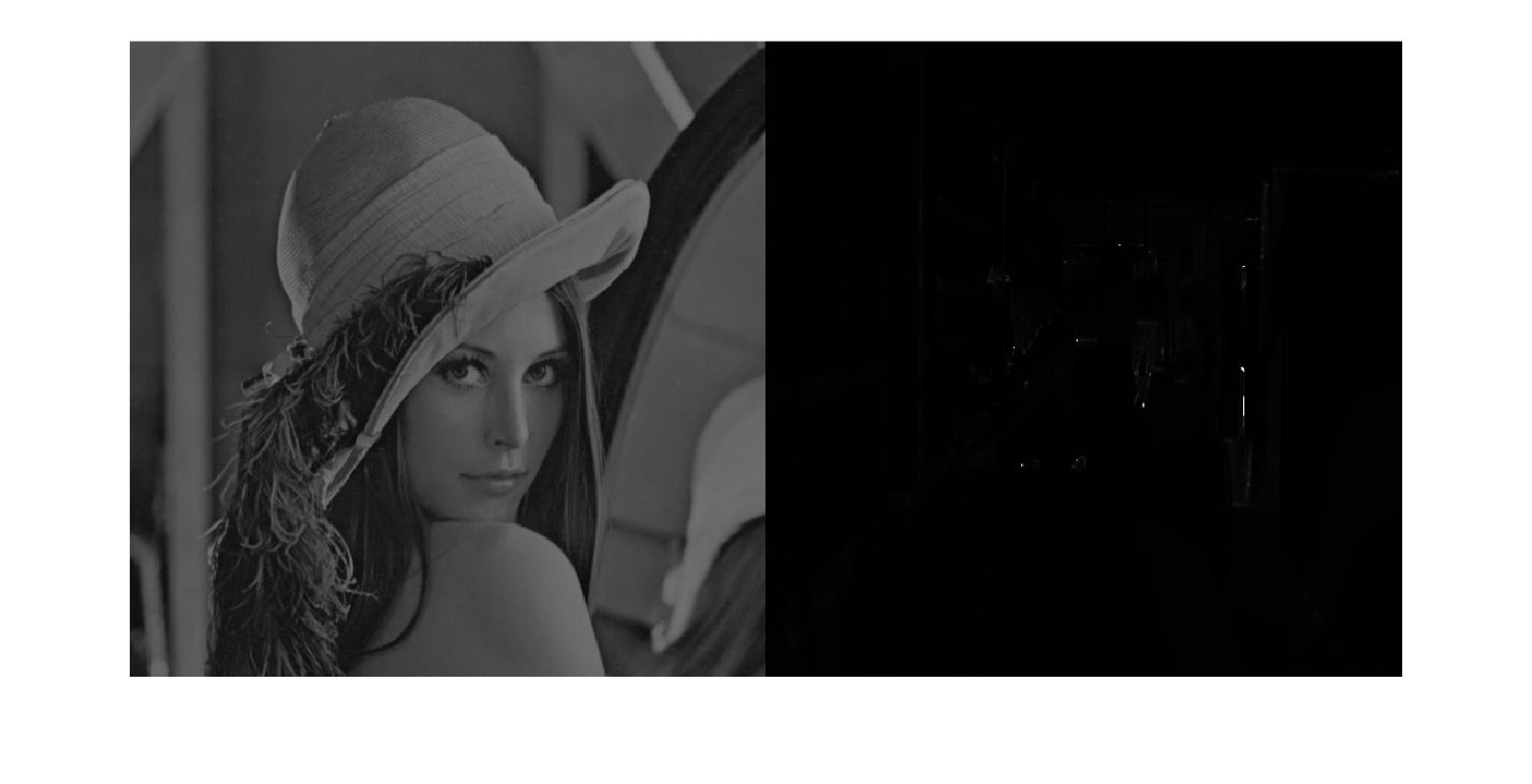
Logical operations

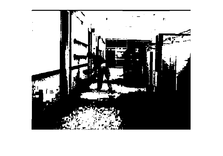
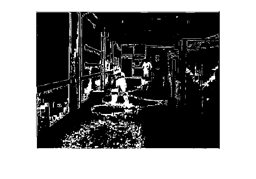
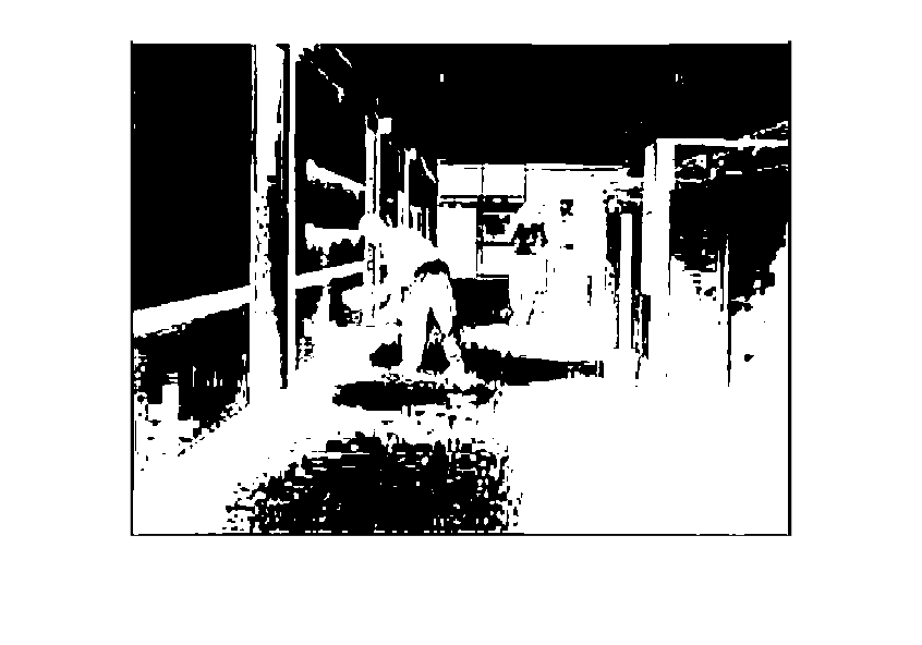
In a binary image, each pixel can belong only to the background or to the object. Therefore, logical operations can be interpreted as operations between sets of pixels: AND corresponds to intersection, OR to union and NOT to complement. This way of thinking will be especially important when mathematical morphology is introduced.

We binarize the images by thresholding

G_bin = G>128;

H_bin = H>128;

We calculate the logical AND (equivalent to the intersection if the objects are defined by 1)

A = and(G_bin,H_bin);

imshow(A

We calculate the logical OR (equivalent to the union if the objects are defined by 1)

O = or(G_bin,H_bin);

imshow(O)

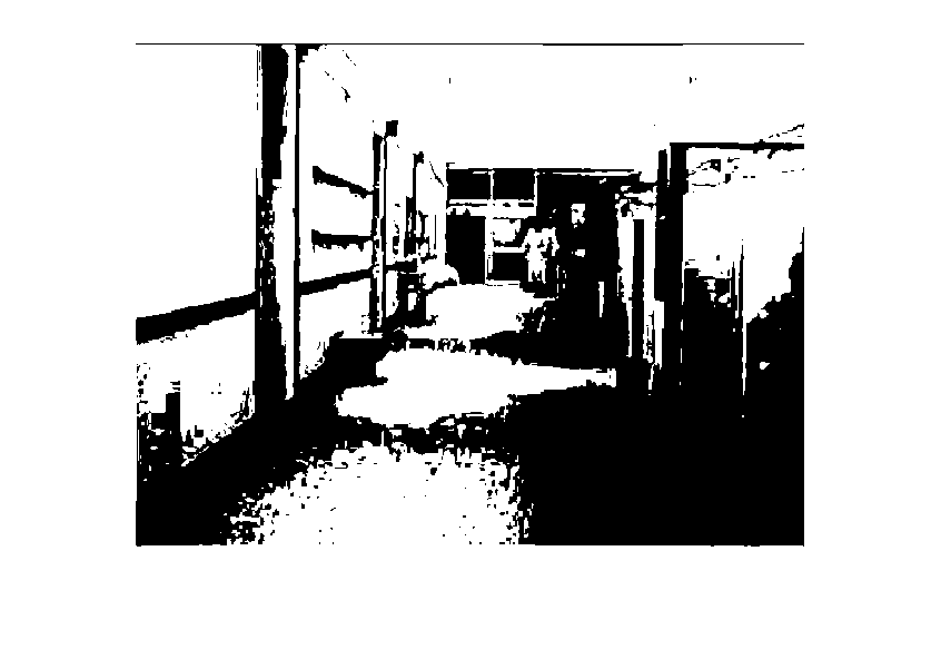
We calculate the logical XOR

X = xor(G_bin,H_bin);

imshow(X)

We calculate the logical NOT

N = not(G_bin);

imshow(N)

Operations with pixel intensity

Intensity transformations are point operations, because each pixel is modified according to its own value and not according to its neighborhood. This type of operation does not move objects or change image geometry; it redistributes gray levels. It can be used to brighten dark regions, compress very bright regions or adjust global contrast.

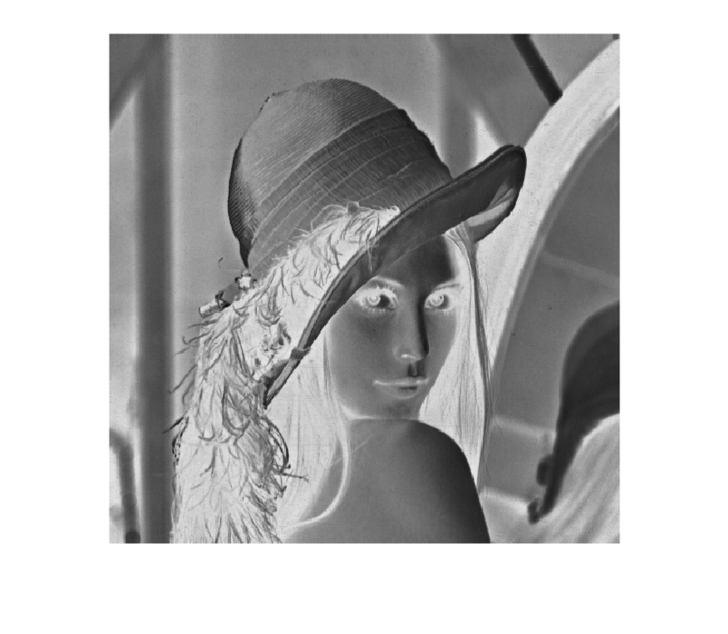
We calculate the negative image

The negative image inverts intensity levels: dark values become bright and bright values become dark. This transformation is simple, but it helps show that many point operations only redistribute values without changing the geometry of the scene.

I_neg = 255-I;

imshow(I_neg)

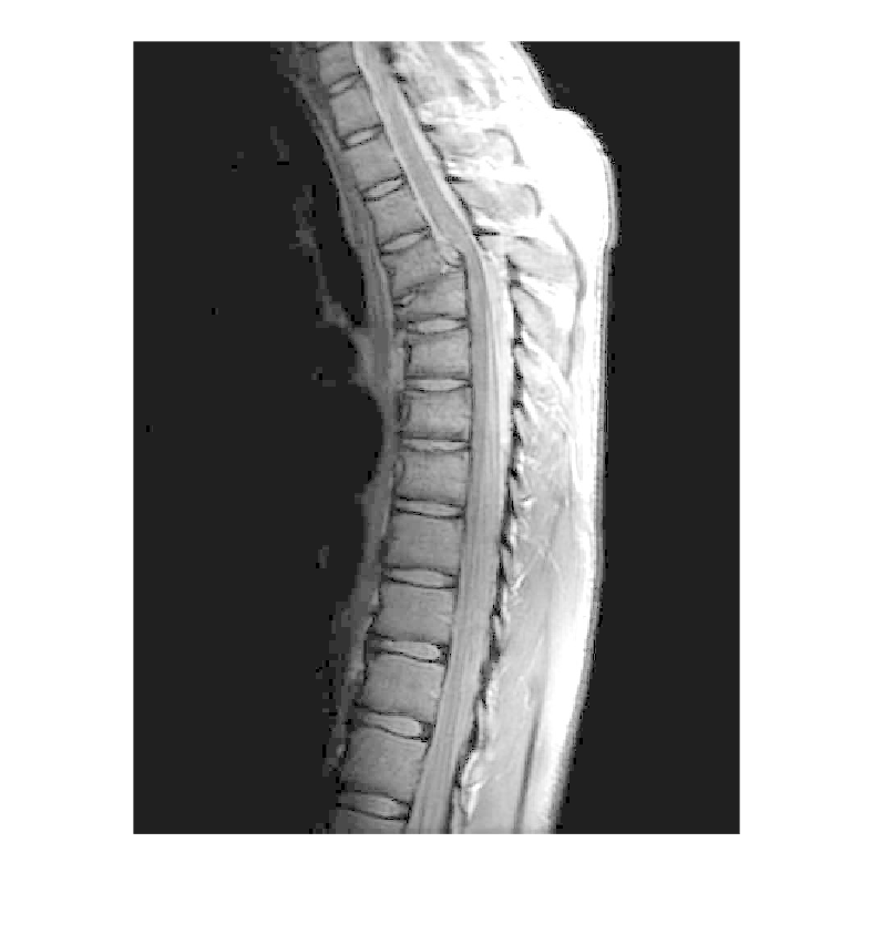
We calculate the logarithmic transformation (with constant c = L-1/log(L) and L gray levels of the image). The logarithmic transformation brightens dark areas while preserving areas that were already bright.

imagen = imread("Imagenes\Espalda.jpg");
imagen = rgb2gray(imagen);
imshow(imagen)

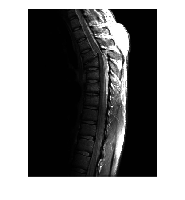
imagen_log = (255/(log(256)))*log(double(imagen) + 1);

imshow(uint8(imagen_log))

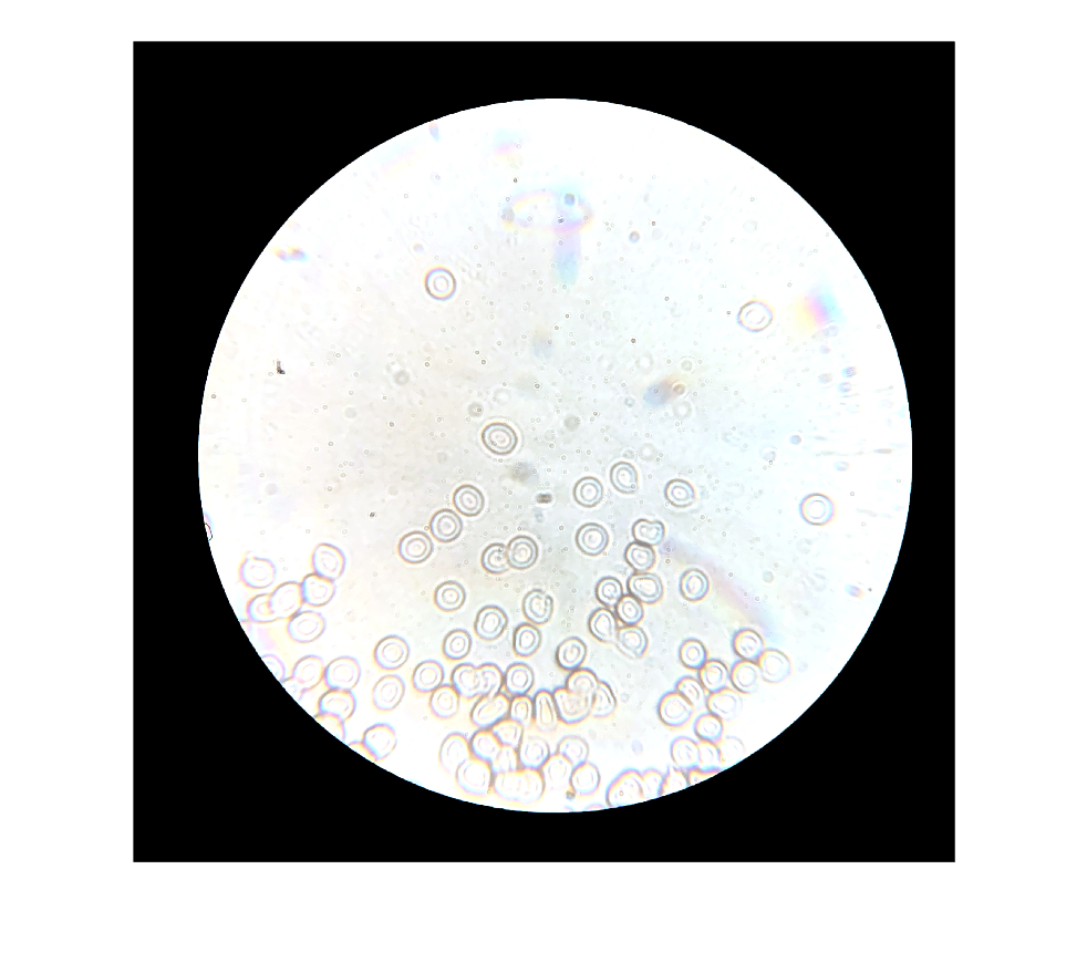
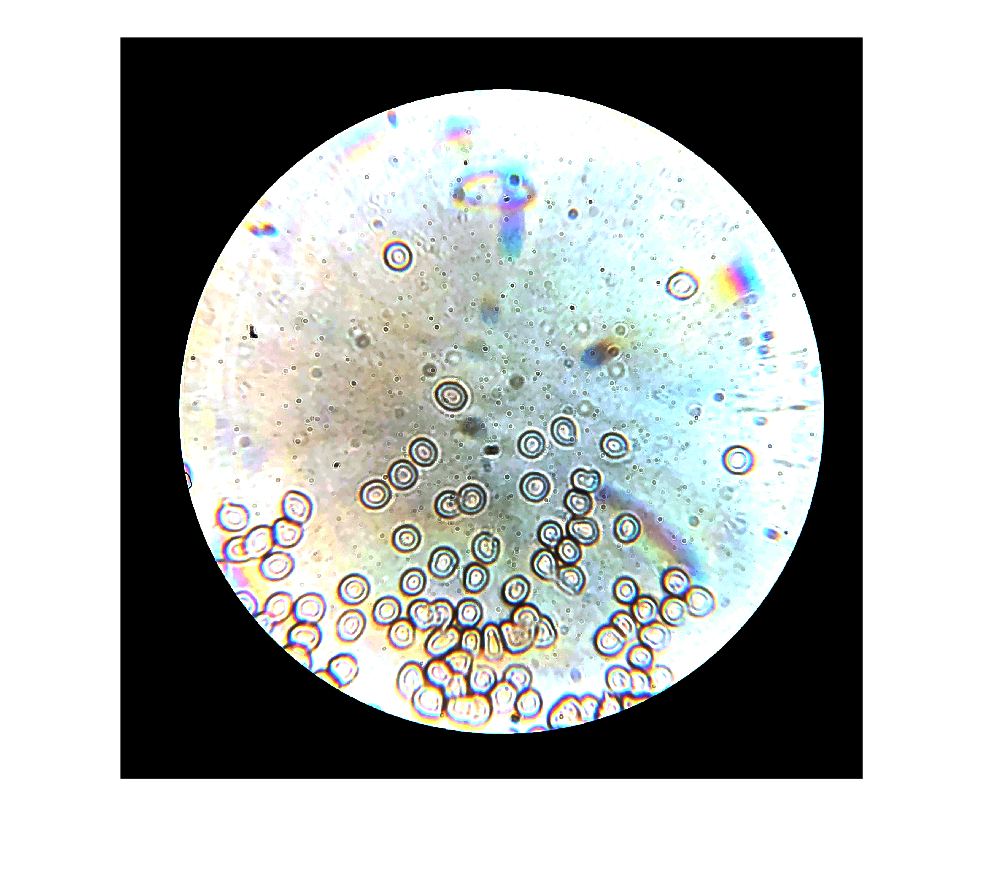
We calculate the exponential transformation (with constant c = L-1/log(L) and L gray levels of the image). The exponential transformation darkens bright areas while preserving areas that were already dark. It is the inverse of the logarithmic transformation.

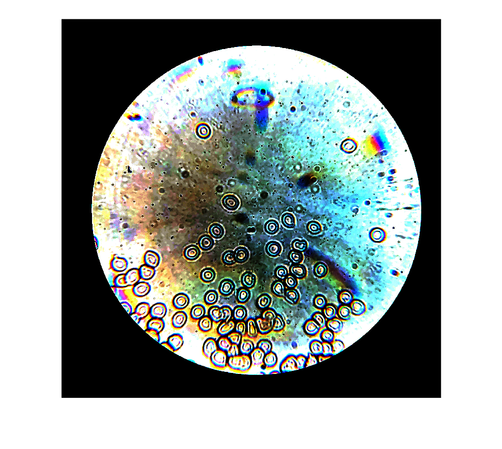
imagen_1 = imread("Imagenes\cells_internet.jpg");

imshow(imagen_1)

imagen_exp = exp((log(256)/255)*double(imagen_1))-1;

imshow(uint8(imagen_exp))

Power-root transformation or gamma correction: It combines and generalizes the logarithmic and exponential transformations

Gamma correction provides flexible control over the relation between input and output intensities. If gamma is smaller than 1, mainly dark regions are brightened; if gamma is greater than 1, mainly bright regions are darkened. It is widely used because it better matches visual perception and display devices.

First step: I transform the intensity values from the interval \(begin:math:display\)0\,255\(end:math:display\) to \(begin:math:display\)0\,1\(end:math:display\)

imagen_1_gamma = (1./255.)*double(imagen_1);

Second step: I define the gamma value and transform

Third step: I transform the intensity values back to the interval \(begin:math:display\)0\,255\(end:math:display\)

gamma = 20;

imagen_1_gamma = uint8(imagen_1_gamma.^gamma * 255);

imshow(imagen_1_gamma)

Histogram expansion and equalization

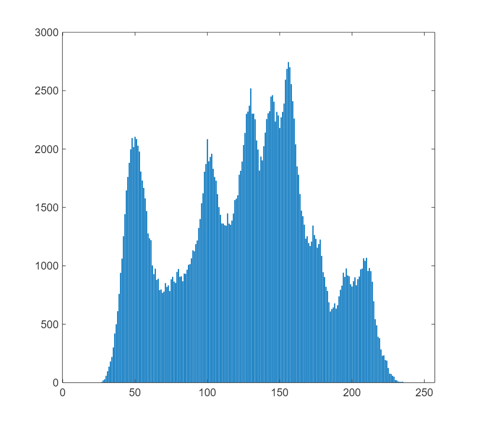
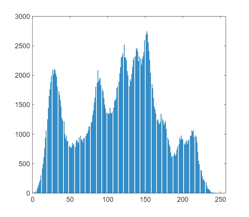
Histogram expansion and equalization try to use the available intensity range more effectively. Expansion spreads values between a minimum and a maximum, while equalization seeks a more uniform distribution. These techniques can improve contrast, but they may also exaggerate noise or give unnatural results when illumination is uneven.

We calculate the histogram

h = imhist(I);
bar(h)

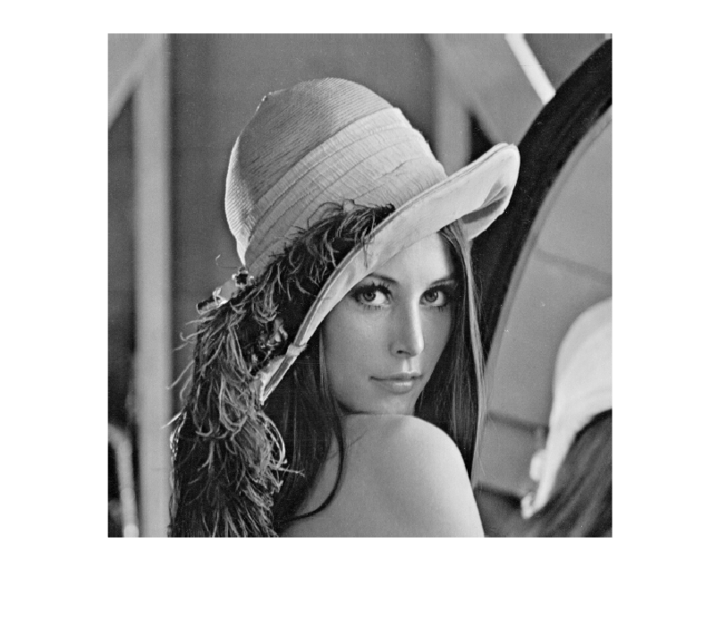
We calculate the maximum and minimum intensity values to expand the histogram

maxi = double(max(max(I)));
mini = double(min(min(I)));
I_exp = 255.*(double(I)-mini)./(maxi-mini);

imshow(uint8(I_exp))

h_exp = imhist(uint8(I_exp));
bar(h_exp)

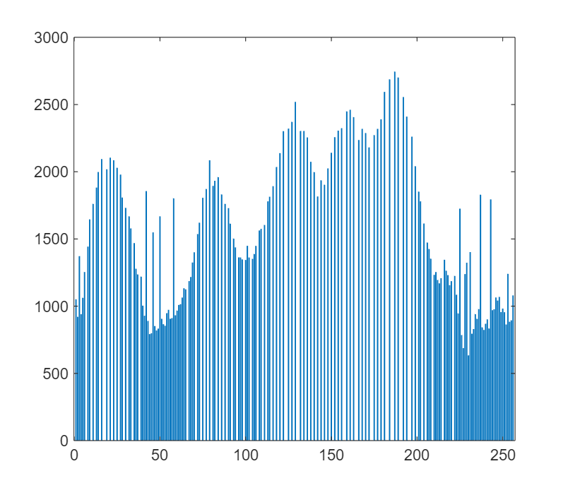
We equalize the histogram, which uniformly distributes the intensity values across the entire interval

I_eq = histeq(I,256);

imshow(I_eq)

h_eq = imhist(I_eq);
bar(h_eq)

Geometric operations

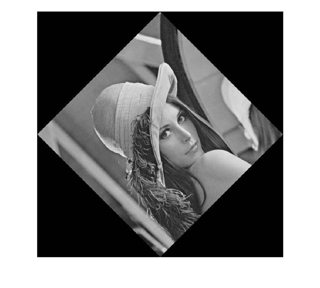
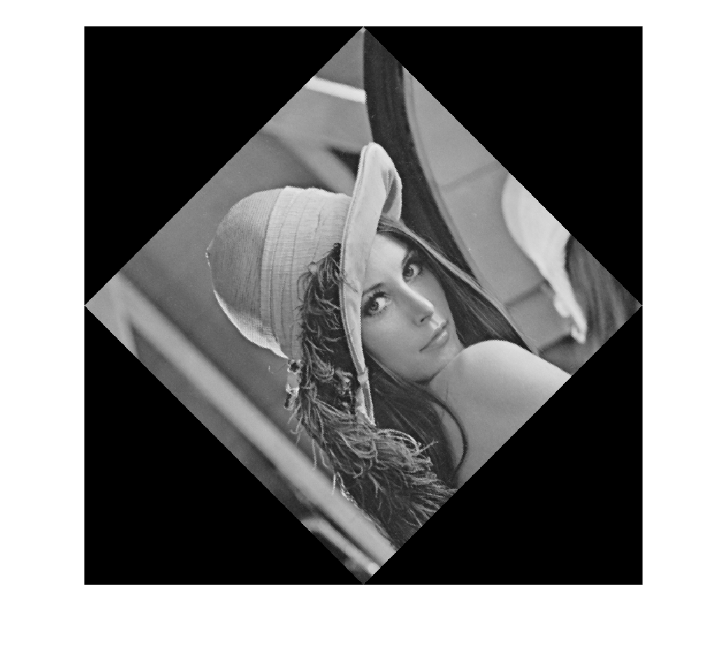
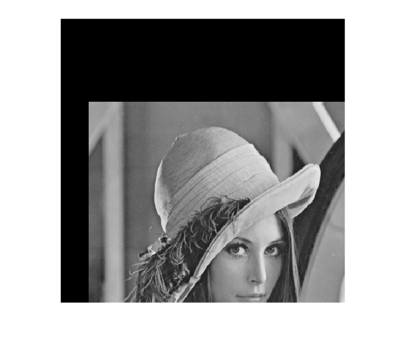
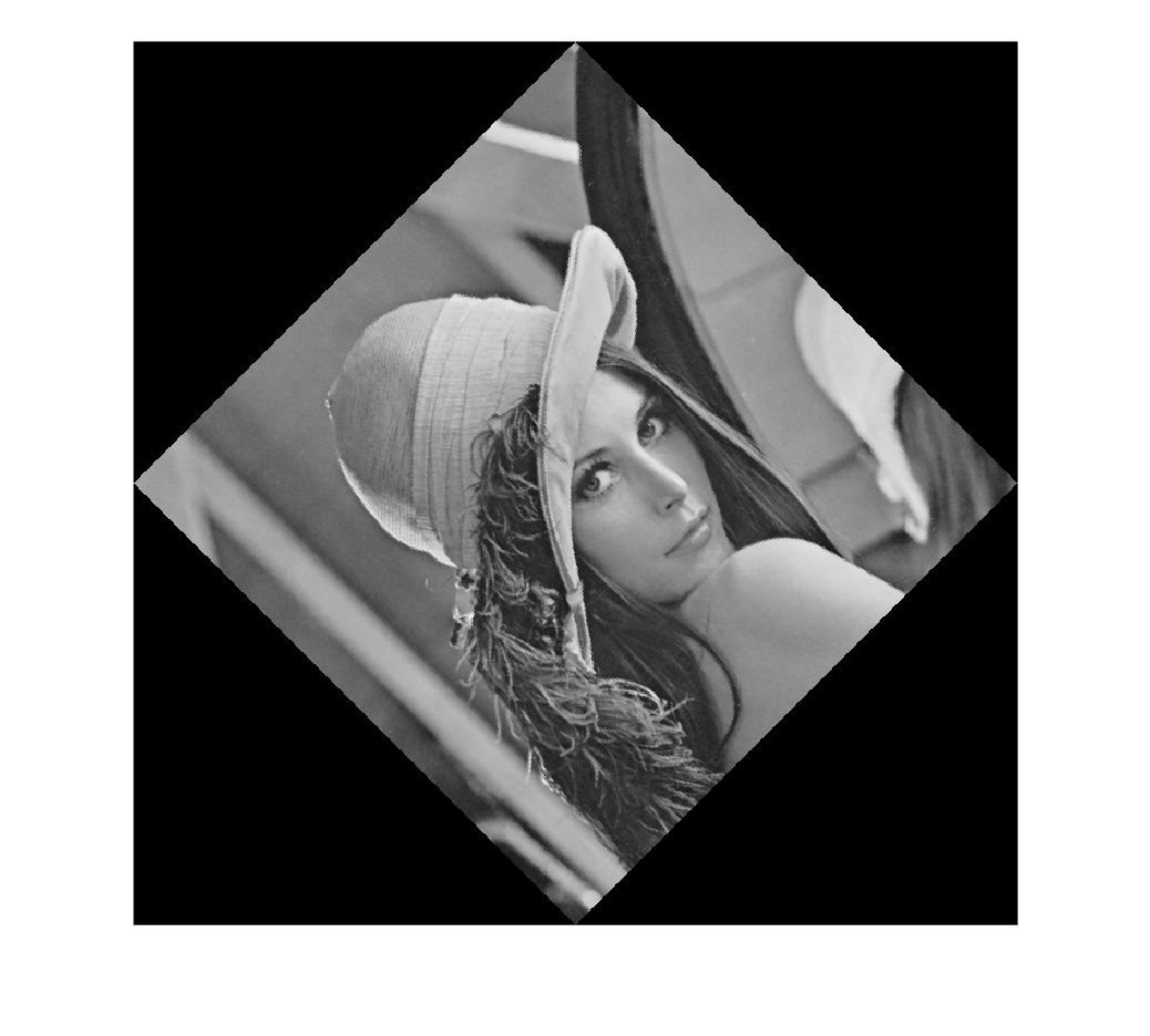
Geometric operations change pixel positions or the apparent size of objects. In rotations, translations or scale changes, the new positions do not always match the discrete pixel grid exactly. For this reason, values must be interpolated, and the interpolation method can influence sharpness, edges and the visual quality of the result.

Rotation by angle theta

I_rot = imrotate(I,45);

imshow(I_rot)

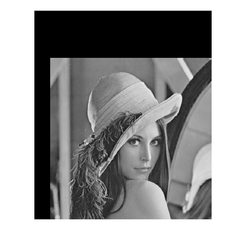
Translation in the (x,y) direction

I_tras = imtranslate(I,[50,150]);

imshow(I_tras)

Translation with full image

I_tras = imtranslate(I,[50,150],'OutputView','full');

imshow(I_tras)

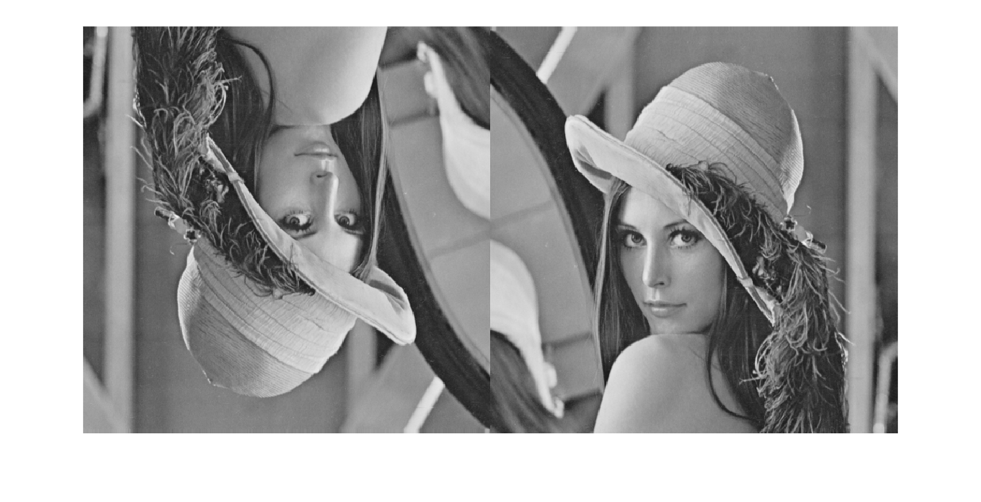
Vertical and horizontal symmetries

I_simv = flip(I,1);
I_simh = flip(I,2);

montage({I_simv,I_simh})

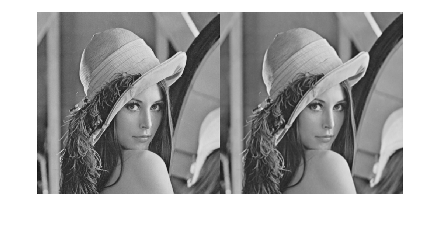
Dilation and reduction by factors d and r.

dilatacion_factor = 2;
reduccion_factor = 0.5;

I_dil = imresize(I,dilatacion_factor);
I_red = imresize(I,reduccion_factor);

montage({I_dil,I_red})

For some of the geometric transformations, the interpolation method must be chosen (e.g., rotations and translations)

Interpolation defines how a pixel value is computed when a geometric transformation places a coordinate between existing pixels. Nearest-neighbor interpolation is fast but can produce jagged edges; bilinear interpolation gives smoother results; and bicubic interpolation usually preserves continuity better, although it is more expensive.

I_rot_n = imrotate(I,45,'nearest');
I_rot_b = imrotate(I,45,'bilinear');
I_rot_bb = imrotate(I,45,'bicubic');

imshow(I_rot_n)

imshow(I_rot_b)

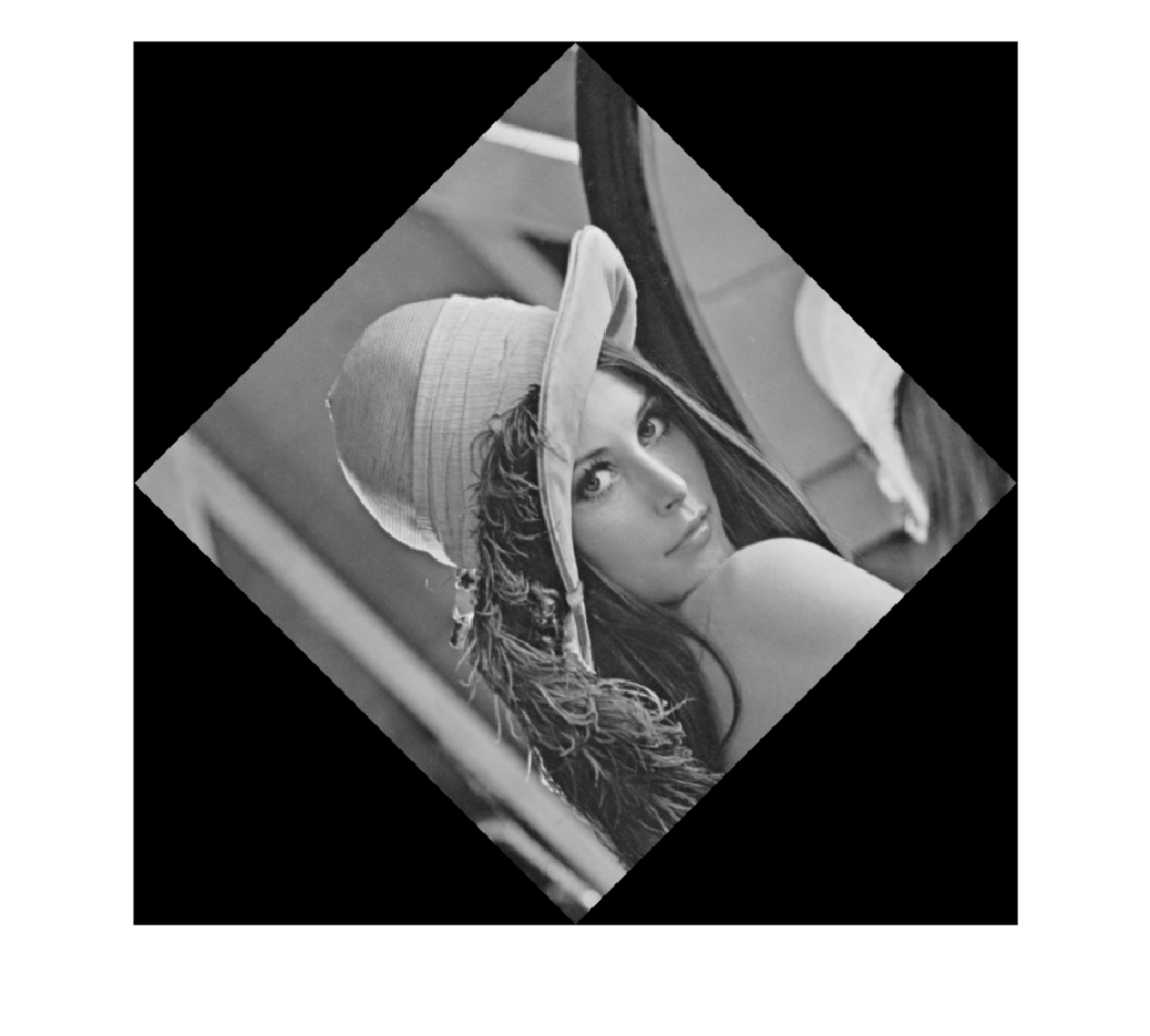
imshow(I_rot_bb)