Tutorial and exercises

This practical works with features that make it possible to describe and compare images. Some are global, such as histograms, because they summarize information from the whole image or a large region. Others are more local, such as vertices or detected lines, because they indicate specific points or structures. All of them help convert visual information into data that are easier to analyze.

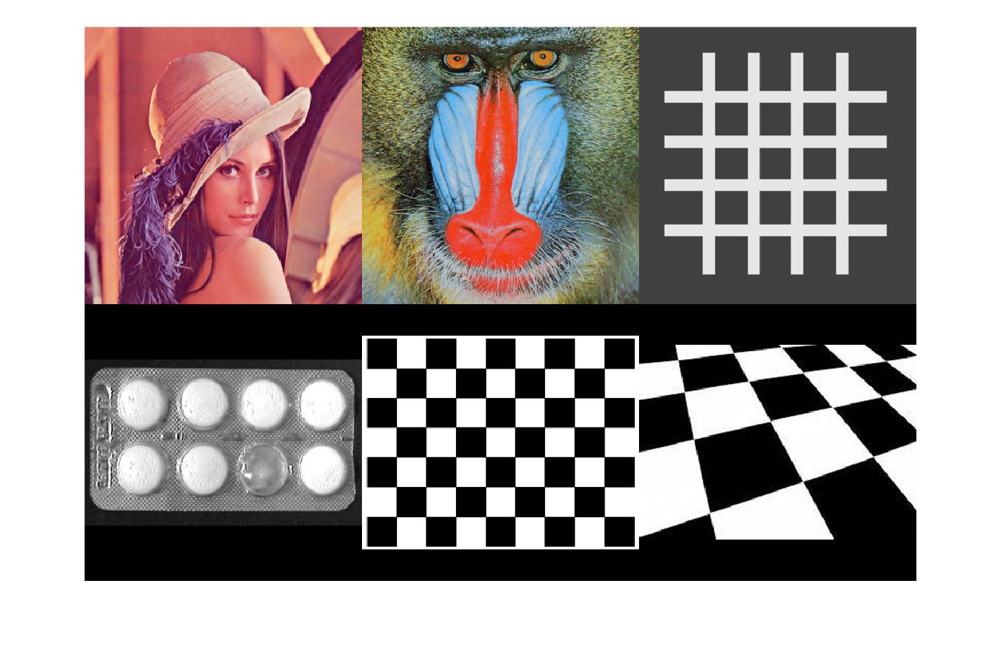
We load the images that we will use in the practical assignment.

lena = imread("Imagenes\lena_color_512.tif");
mandril = imread("Imagenes\mandril_color.tif");
malla = imread("Imagenes\patron_malla.jpg");
textura = imread("Imagenes\astablet.tif");
chessboard = imread("Imagenes\chessboardpattern.jpg");
chessboard_inclinado = imread("Imagenes\esquinas_perspectiva.jpg");

malla = rgb2gray(malla);
chessboard_inclinado = rgb2gray(chessboard_inclinado);

montage({lena,mandril,malla,textura,chessboard,chessboard_inclinado})

Histogram-based features

A color histogram indicates how the values of the color channels are distributed. It is useful for describing the general appearance of an image, for example whether dark, bright or specific colors dominate. However, the histogram does not preserve spatial information: two images may have the same histogram while showing objects arranged in completely different ways.

Color histogram

First example: Lena image

We separate the image into the three color channels

red = lena(:,:,1);
green = lena(:,:,2);
blue = lena(:,:,3);

And we obtain the histograms of each channel

h_red = imhist(red);
h_green = imhist(green);
h_blue = imhist(blue);

bar(h_red)

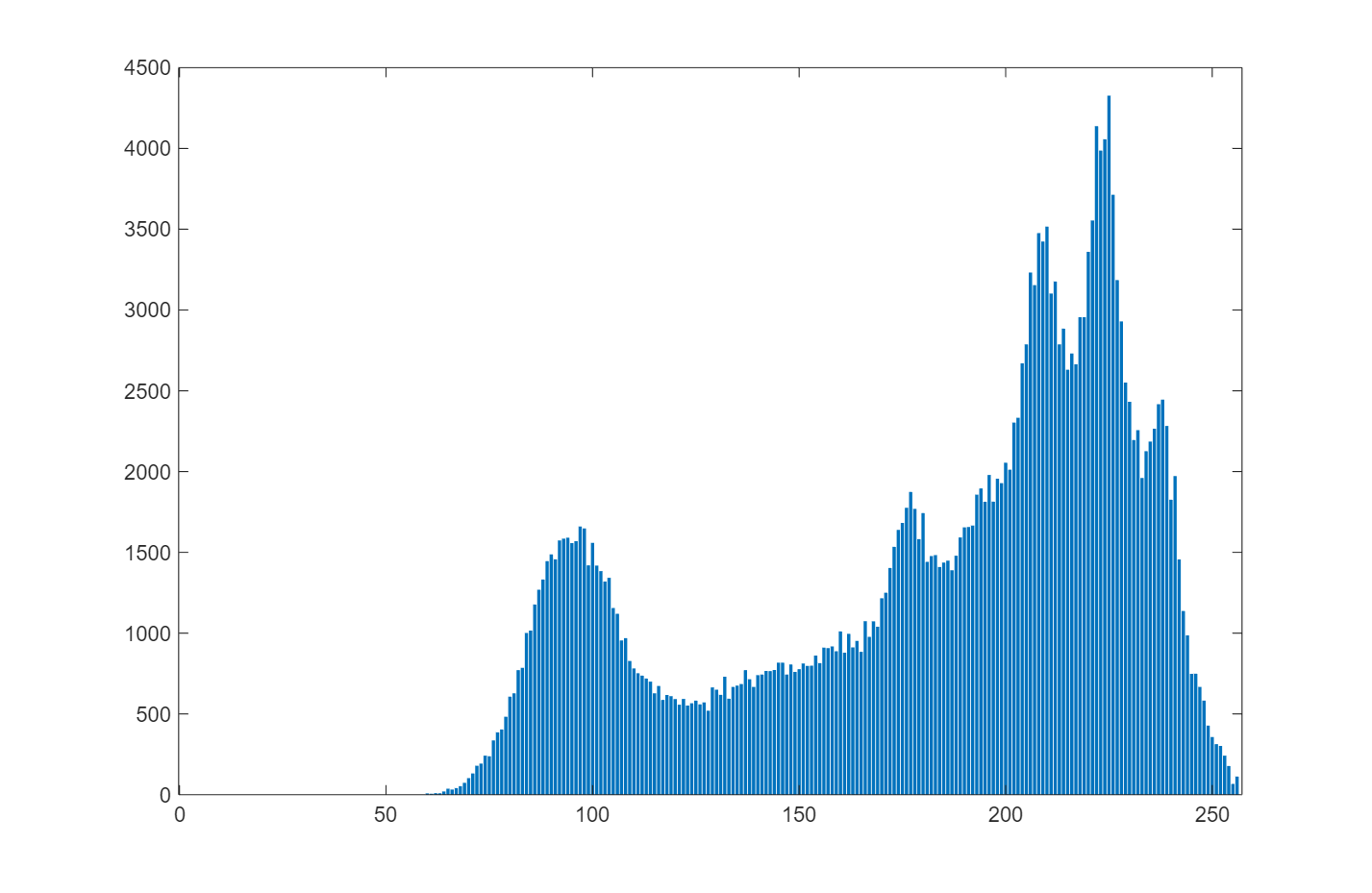
bar(h_green)

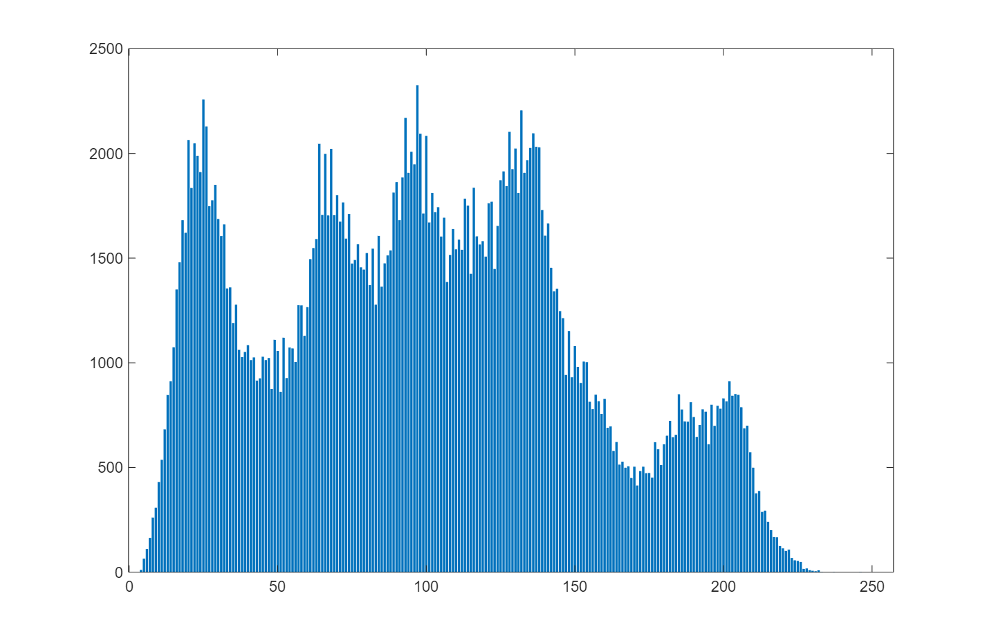
bar(h_blue)

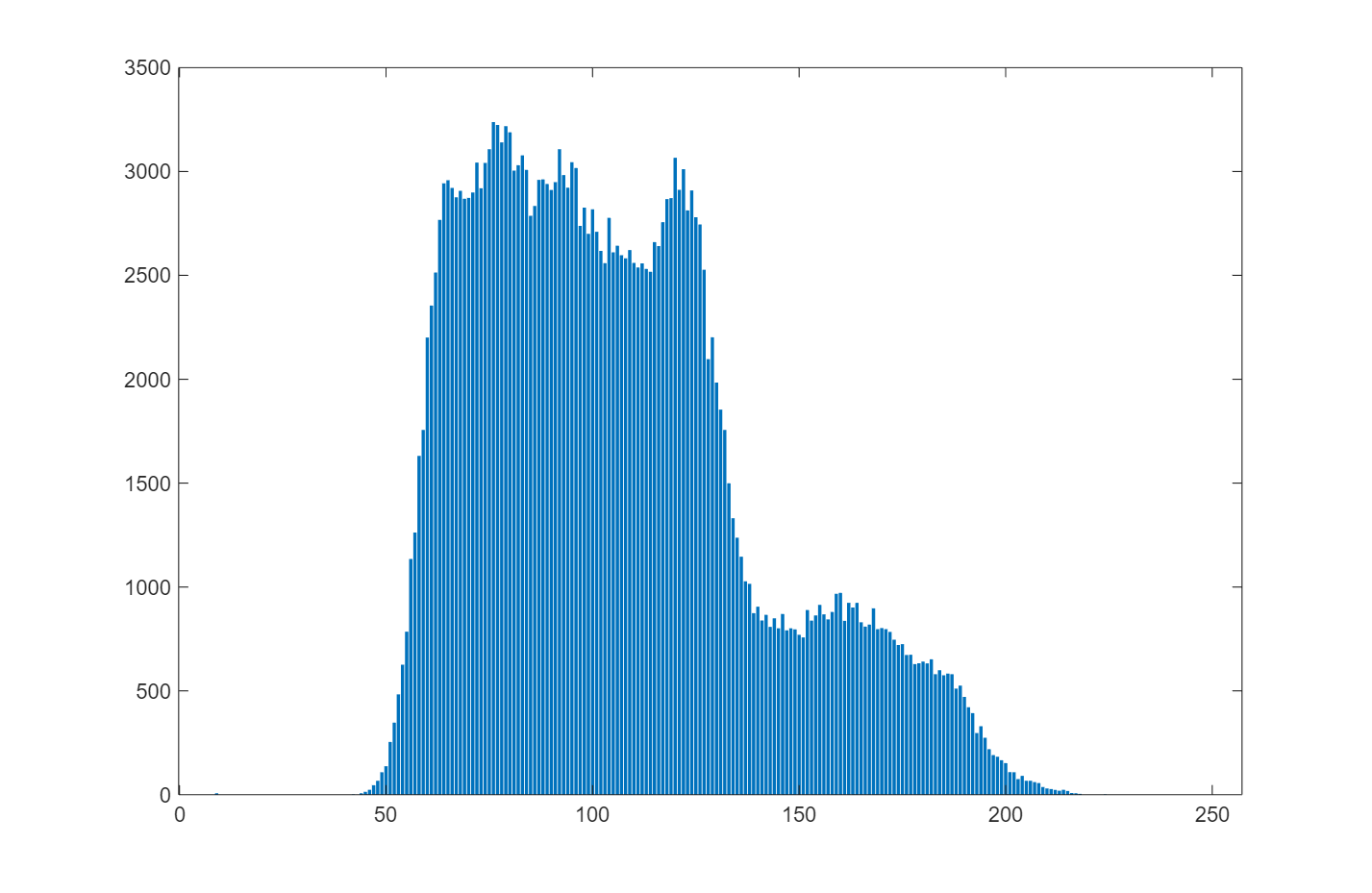
Another example: Mandrill image

red = mandril(:,:,1);
green = mandril(:,:,2);
blue = mandril(:,:,3);

h_red = imhist(red);
h_green = imhist(green);
h_blue = imhist(blue);

bar(h_red)

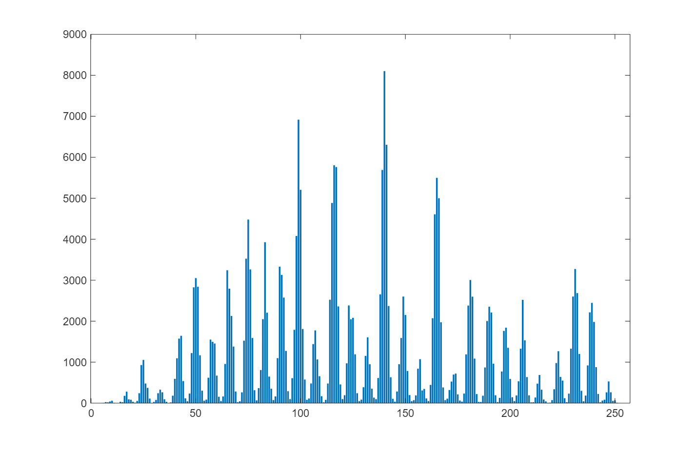
bar(h_green)

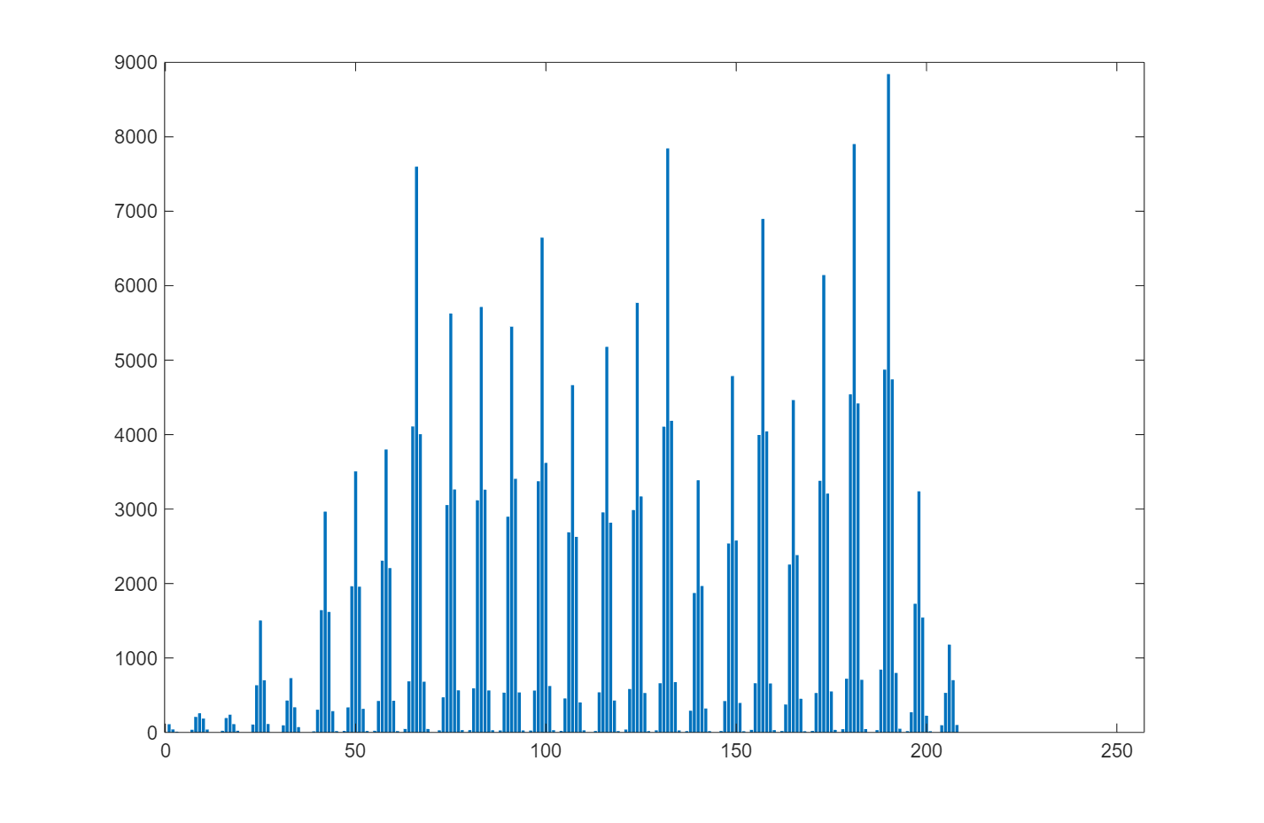
bar(h_blue)

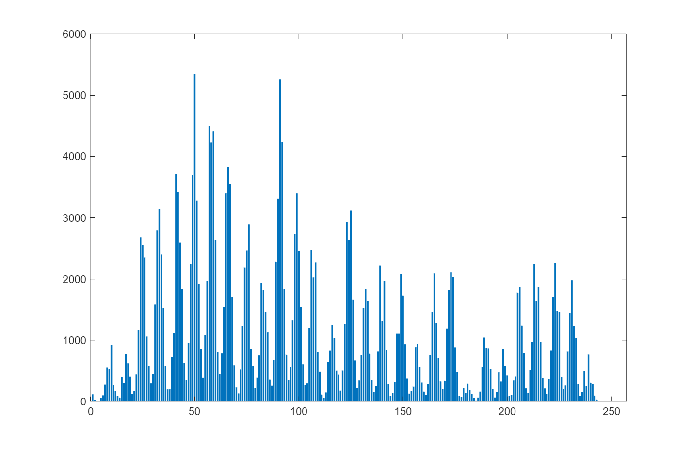
We calculate the similarity measures to compare histograms. To simplify, we are going to compare only one histogram per image.

Comparing histograms means measuring how similar two intensity or color distributions are. Euclidean distance treats differences directly, chi-square gives more importance to relative differences, and Jeffrey divergence compares distributions in a more symmetric way. No metric is universally best; it depends on what should be considered similar.

lena_gris = rgb2gray(lena);
mandril_gris = rgb2gray(mandril);

h_lena = imhist(lena_gris);
h_mandril = imhist(mandril_gris);

We normalize the histogram

Histogram normalization is necessary when comparing images of different sizes or with different numbers of pixels. Without normalization, a larger image could give higher values simply because it contains more pixels. After normalization, the comparison focuses more on the shape of the distribution and less on the absolute number of samples.

h_lena_n = h_lena/numel(lena_gris);
h_mandril_n = h_mandril/numel(mandril_gris);
bar(h_lena_n)

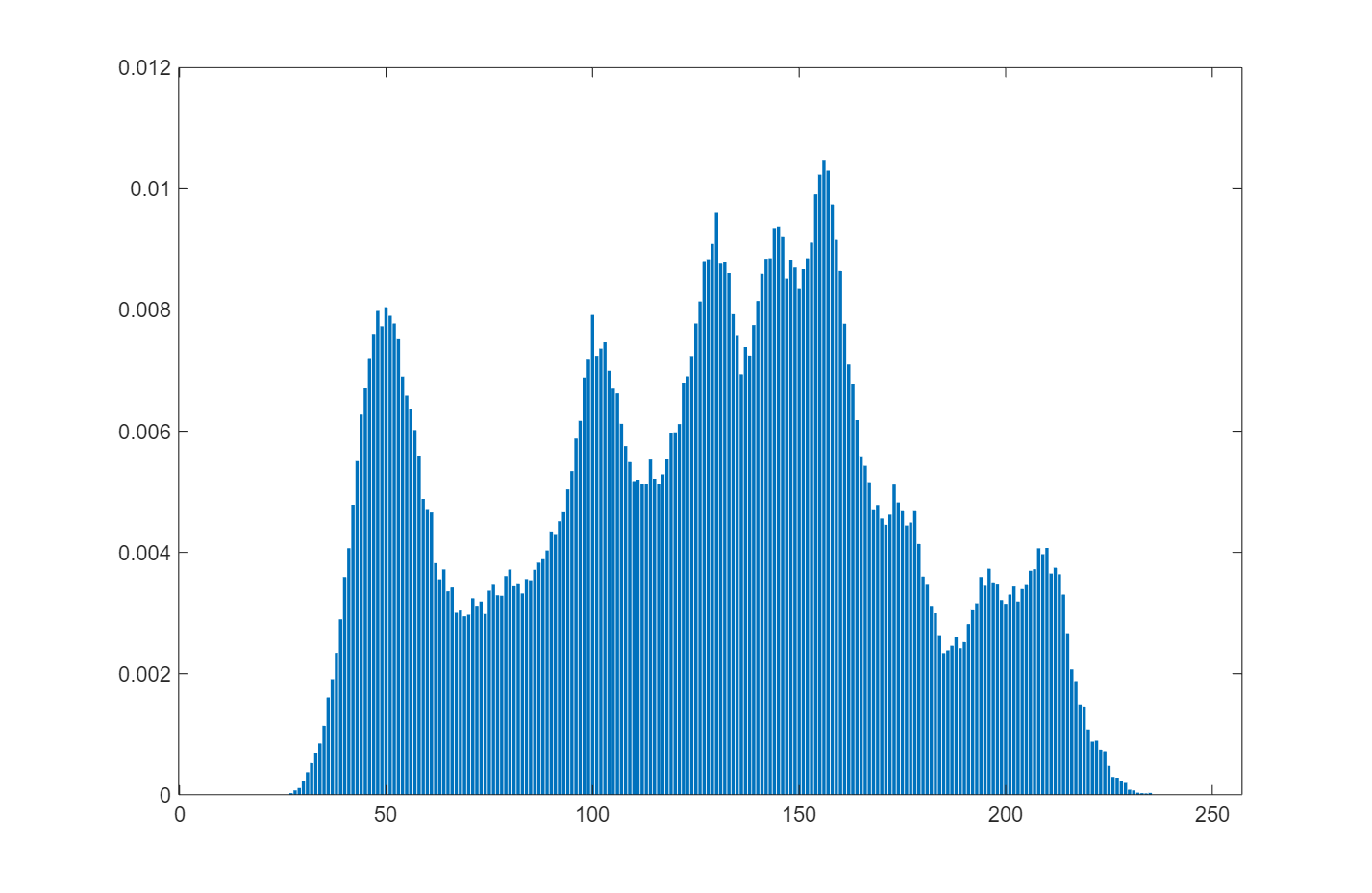
bar(h_mandril_n)

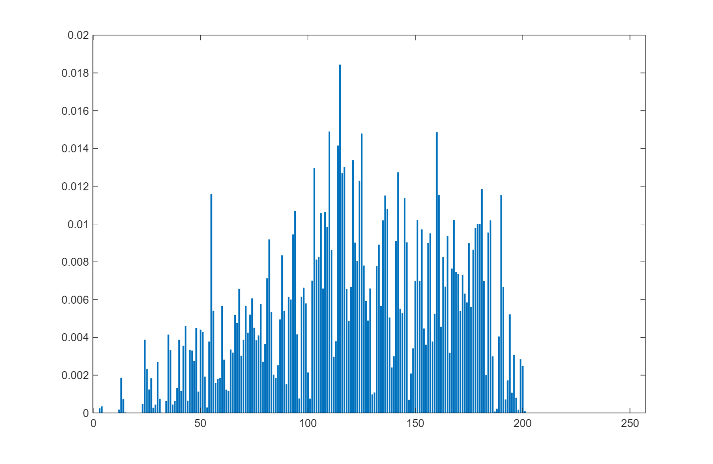
Euclidean distance

dist_euclidea = sqrt(sum((h_lena_n - h_mandril_n).^2))

dist_euclidea = 0.0533

Chi-square distance

dist_xicuadrado = sum(((h_lena_n - h_mandril_n).^2) ./ (h_lena_n + h_mandril_n + eps))

dist_xicuadrado = 0.2997

Jeffrey divergence distance

divergence_jeffrey = sum(h_lena_n.*log((h_lena_n./(h_mandril_n + eps))+eps))

divergence_jeffrey = 2.1436

Histogram of oriented gradients

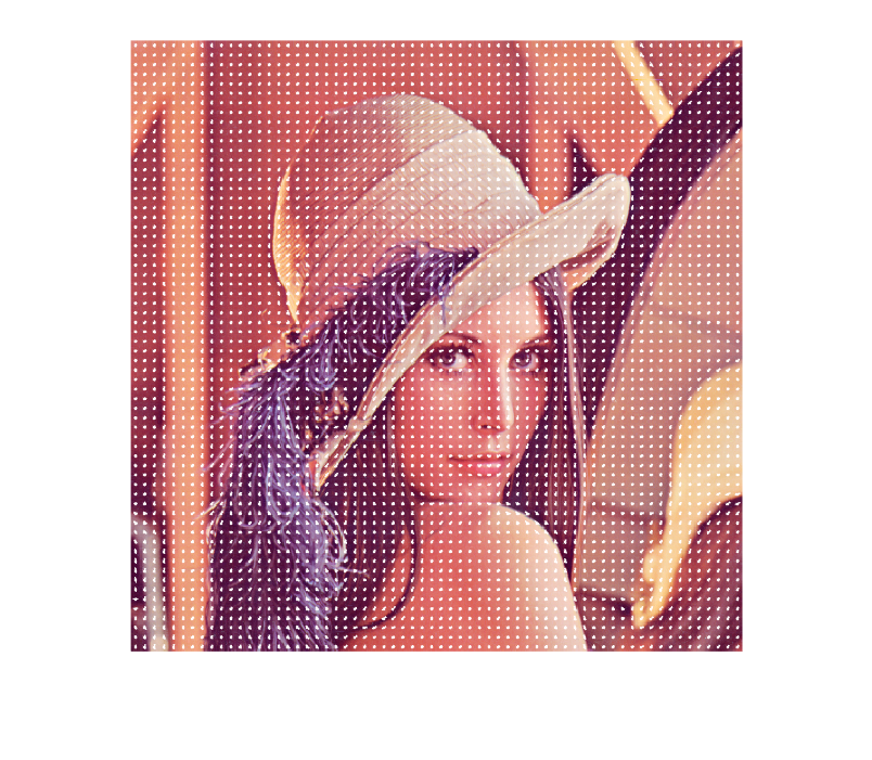
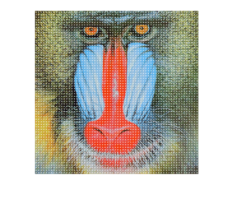
The histogram of oriented gradients, or HOG, describes the distribution of gradient directions in small image regions. Since the gradient is strong at edges, this descriptor summarizes information about contours and local shapes. For many years it was widely used in object detection, especially before convolutional networks became common.

First example: Lena image

Command: extractHOGFeatures

[feature_vector,hog] = extractHOGFeatures(lena);

imshow(lena); 
hold on;
plot(hog);
hold off

Another example: Mandrill image

[feature_vector_mandril,hog_mandril] = extractHOGFeatures(mandril);
imshow(mandril);
hold on
plot(hog_mandril);
hold off

Hough transform-based features

The Hough transform is a technique for detecting simple geometric shapes, such as lines or circles. The idea is that each edge point votes for the shapes that could pass through it. When many points vote for the same set of parameters, it is likely that a real shape is present in the image. This makes it possible to detect structures even when edges are not perfect or are partially interrupted.

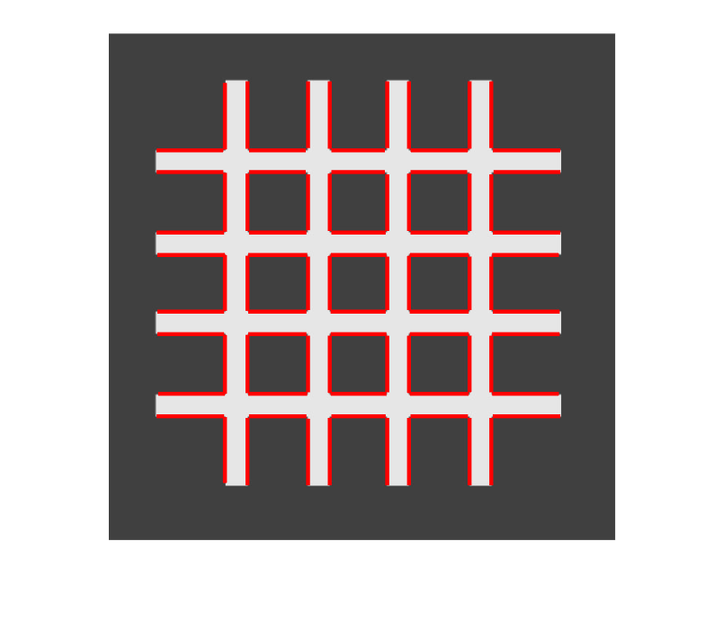
Obtaining lines via the Hough transform

First we obtain the image edges

The Hough transform is usually not applied to the whole image, but to an edge image. This reduces the number of voting points and focuses the process on pixels that are likely to belong to lines or contours.

malla_edge = edge(malla,"canny");

Command: hough. It gives as output the discretization of the Hough plane H, with the values of theta T and rho R

[H,T,R] = hough(malla_edge);

We calculate the peaks (points with higher value) in that discretization of the Hough plane. In particular, we keep the 16 highest-value peaks that are above 35% of the maximum value.

A peak in Hough space indicates that many edge points are compatible with the same line. Selecting only the strongest peaks avoids considering weak lines or lines caused by noise. The threshold controls how many structures are kept.

P = houghpeaks(H, 16,'threshold',ceil(0.35*max(H(:))));

We calculate the lines with those peaks and their associated theta and rho values (which define the corresponding lines).

lines = houghlines(malla_edge,T,R,P);

imshow(malla)
hold on

for k = 1:length(lines)

    xy = [lines(k).point1; lines(k).point2];
    plot(xy(:,1),xy(:,2),'LineWidth',2,'Color','red');

end
hold off

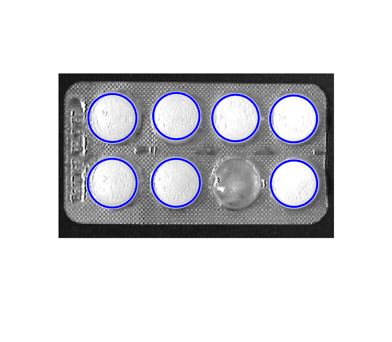
We obtain the circles in the image via the Hough transform. To do this, we use the imfindcircles command, which searches for circles with a radius whose value is within the range defined as the second input.

To detect circles, the method searches for vote accumulations compatible with a center and a radius. The radius range is important: if it is too wide, false positives increase; if it is too restrictive, real circles may be missed. This range should therefore be related to the expected size of the objects.

[centers, radii] = imfindcircles(textura,[10 30]);
imshow(textura)
viscircles(centers, radii,'EdgeColor','b');

Vertices

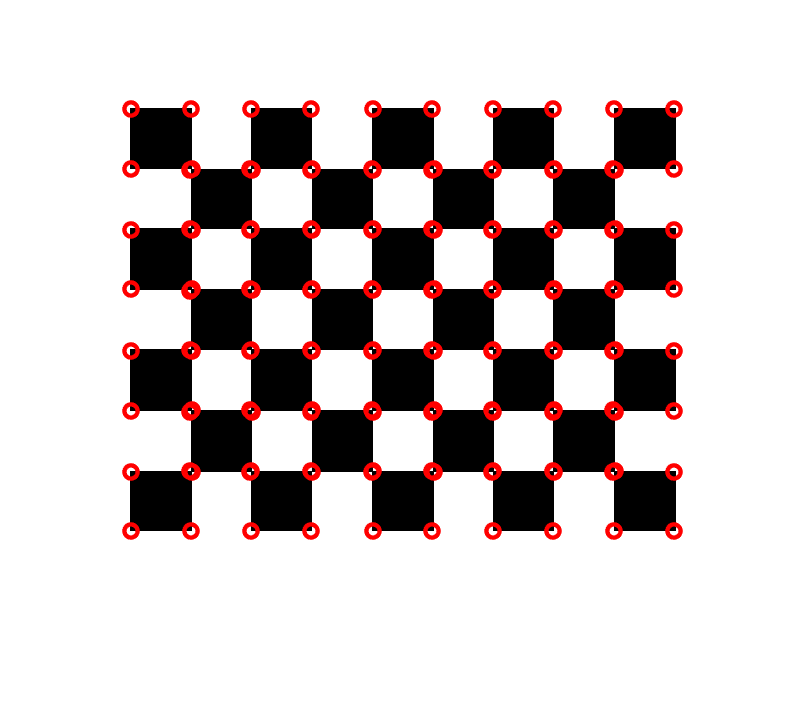
A vertex or corner is a point where the image changes significantly in more than one direction. This type of point can be localized more precisely than a straight edge, because an edge can move along its own direction without changing much. Corners are therefore useful as interest points for image registration, tracking and image matching.

The Harris detector is used to identify corners and vertices in the images.

The Harris detector analyzes how intensity changes inside a small window when that window is shifted. If the change is large in all directions, the central point is considered a good corner. If the change is large only in one direction, it is probably an edge. To obtain more reliable results, only the points with the strongest response are usually kept.

corners = detectHarrisFeatures(chessboard);

imshow(chessboard); 
hold on
plot(corners.Location(:,1),corners.Location(:,2),'o','Color','r','LineWidth',2);
hold off

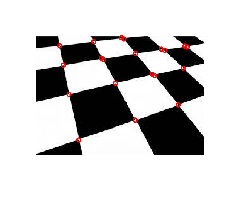
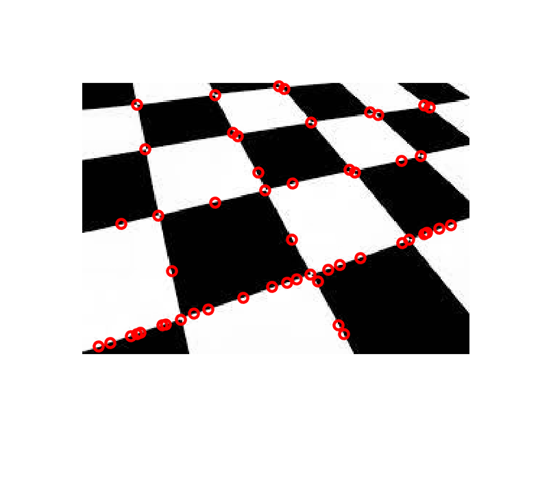
Another example. Note that in this case several false positives are detected. A more detailed analysis shows that their metric is very low, so they can be easily removed by selecting the strongest ones, that is, those with a more robust detection.

corners_alt = detectHarrisFeatures(chessboard_inclinado);

imshow(chessboard_inclinado); 
hold on
plot(corners_alt.Location(:,1),corners_alt.Location(:,2),'o',"color",'r','LineWidth',2);
hold off

imshow(chessboard_inclinado)

strongest = corners_alt.selectStrongest(20);

hold on
plot(strongest.Location(:,1),strongest.Location(:,2),'o','color','r','LineWidth',2)
hold off