Tutorial and exercises

Segmentation consists of dividing an image into regions that have meaning for the task. These regions may correspond to objects, background, edges or parts of a scene. There is no single method that works well for all images, because each technique is based on a different assumption: similar intensities, abrupt changes, connectivity or morphological properties.

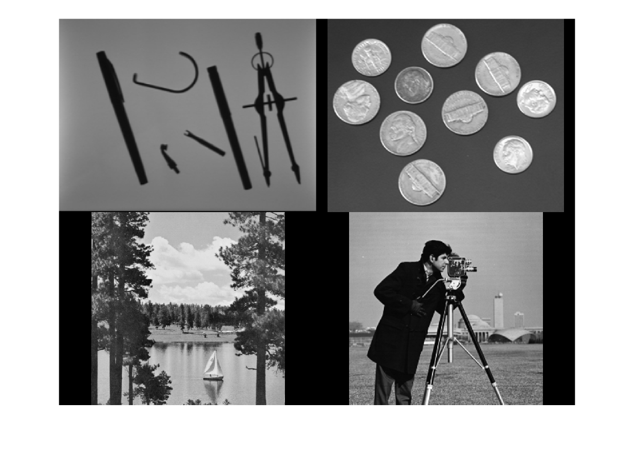
We load the images that we will use during this part of the practical session.

objetos = imread("Imagenes\objects.tif");
monedas = imread("Imagenes\coins.png");
lake = imread("Imagenes\lake.tif");
cameraman = imread("Imagenes\cameraman.tif");

Since lake has two channels, we take one!

lake = lake(:,:,1);

We display the images

montage({objetos,monedas,lake,cameraman})

Segmentation by thresholding

Threshold-based segmentation is one of the simplest techniques. It consists of choosing an intensity value and classifying pixels according to whether they are above or below that value. It works especially well when the object and the background have clearly different intensities. However, it may fail when there are shadows, reflections or nonuniform illumination.

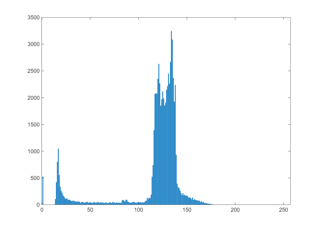
Threshold selection through direct study of the histogram

When a threshold is chosen manually, the histogram serves as a guide. If two groups of intensities are well separated, the threshold can be placed in the valley between them. If the groups overlap, the result will be more sensitive to errors.

h_objetos = imhist(objetos);

bar(h_objetos)

Threshold (estimated visually from the histogram)

T=75;

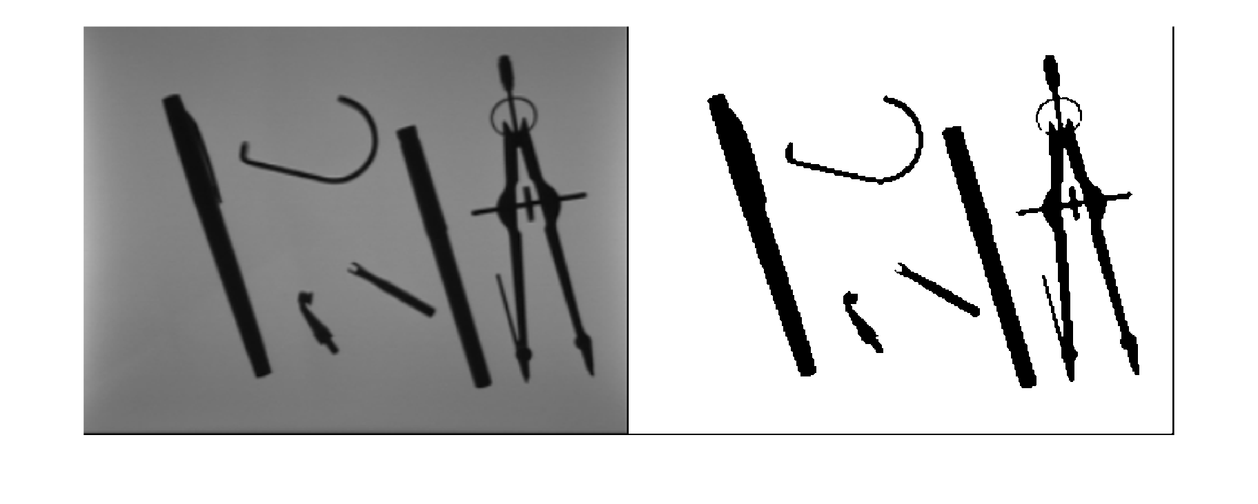
objetos_bin = objetos>T;

The imbinarize command can also be used if we use T/255.

montage({objetos,objetos_bin})

Another example

h_lake = imhist(lake);

bar(h_lake)

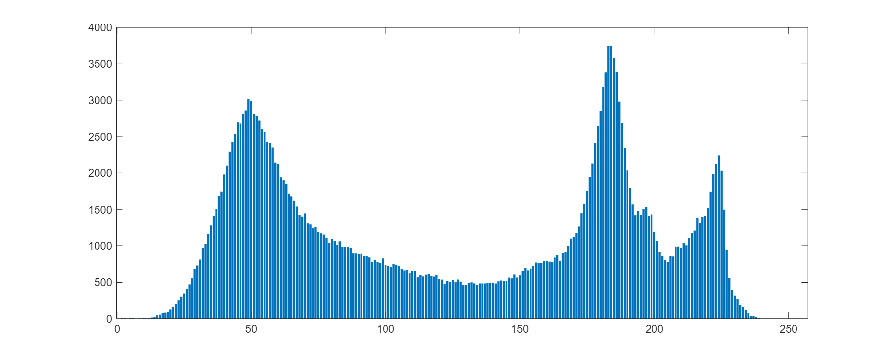
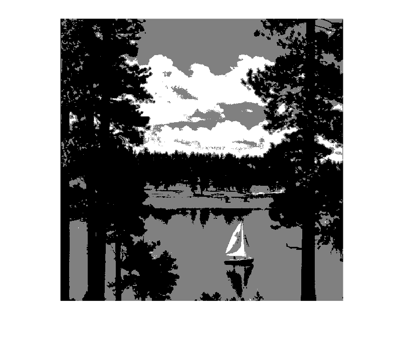
Thresholds (estimated visually from the histogram)

T1 = 130;
T2 = 205;

lake_bin = imquantize(lake,[0,T1,T2,255]);

imshow(lake_bin,[])

Otsu method

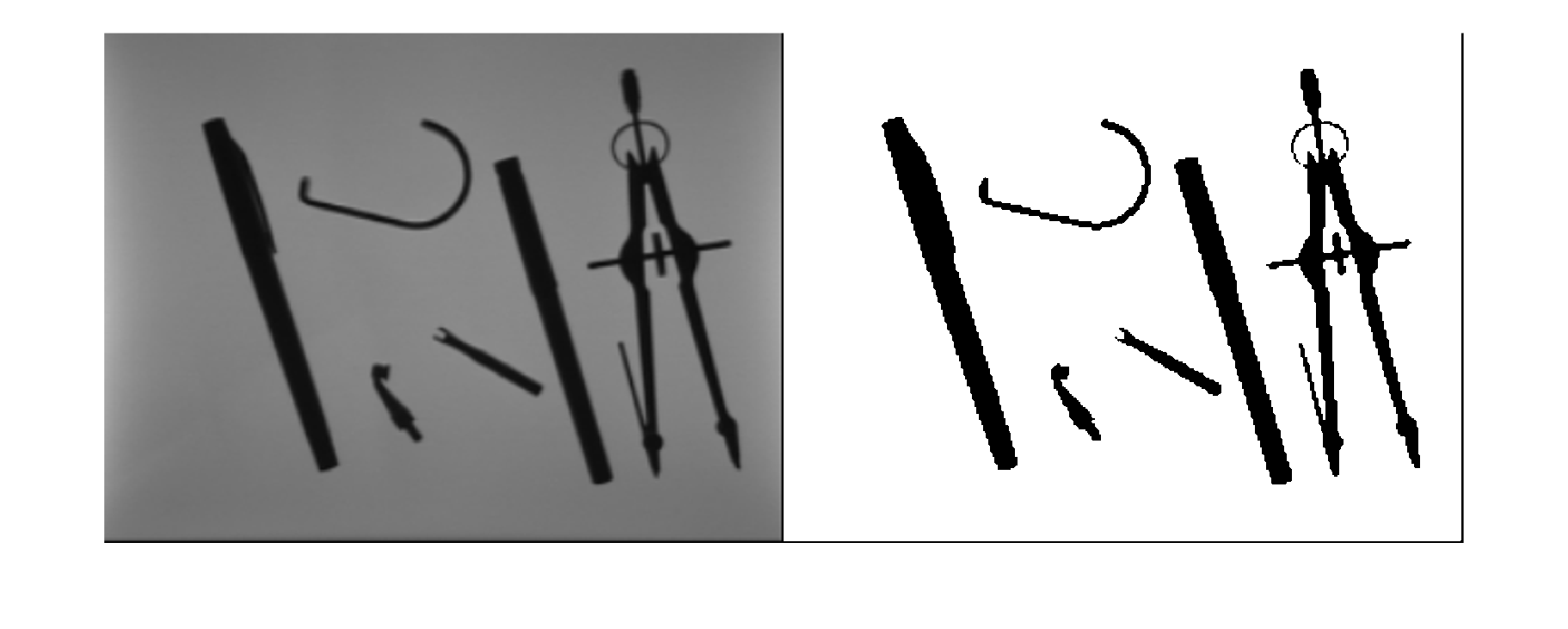
Otsu's method automatically computes a threshold from the histogram. The idea is to separate pixels into two classes so that each class is as compact as possible and the two classes are well separated. Since it is a global method, it uses a single threshold for the whole image; therefore, it does not always work well when illumination changes across the image.

T_otsu = graythresh(objetos);

objetos_bin = imbinarize(objetos,T_otsu);

montage({objetos,objetos_bin})

Labeling and coloring connected components

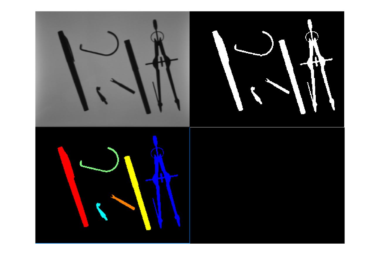
After binarization, connected components are often identified. A connected component is a set of foreground pixels joined according to a neighborhood rule. This rule may consider only horizontal and vertical connections, or also diagonal connections. The chosen connectivity can change the number of detected objects.

First we apply not(objetos), since we want the connected components to be white on a black background.

objetos_neg = not(objetos_bin);

We use the bwlabel command, which labels the connected components in a binary image.

comps_conexas = bwlabel(objetos_neg);

To visualize the result (which is completely optional), we use label2rgb, which colors each connected component according to a color palette.

objetos_col = label2rgb(comps_conexas,"jet","k","shuffle");

montage({objetos,objetos_neg,objetos_col})

Segmentation methods based on edge detection

Edge-based methods look for points where intensity changes abruptly. These points often indicate the boundary between objects or between different regions of the scene. However, a detected edge does not always form a closed contour, and therefore does not always directly define a segmented region. For this reason, edge detection is often combined with other postprocessing steps.

Line detection using the Laplacian

A Laplacian kernel designed with a specific orientation can respond strongly to linear structures. In this example it is used to highlight vertical lines, that is, regions where intensity changes in a way compatible with that structure.

lineas = imread("Imagenes\lineas.png");
lineas = rgb2gray(lineas);

Laplacian kernel to detect vertical lines

w_verticales = [-1,2,-1;-1,2,-1;-1,2,-1];

lineas_filt = abs(imfilter(lineas,w_verticales));

Threshold to discriminate the calculated lines and remove the weakest ones (which will probably either not be lines or not be vertical lines).

maxi = max(lineas_filt(:));

lineas_filt_bin = lineas_filt>=maxi;

montage({lineas,lineas_filt,lineas_filt_bin})

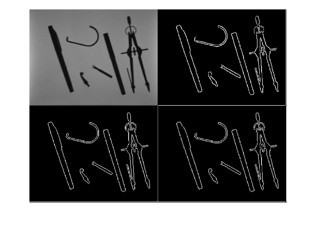
The edge command is used for edge detection with the digital gradient and as an alternative to the specific Roberts/Sobel and Prewitt commands obtained with the fspecial command.

The edge function groups several edge detectors under the same interface. This makes it possible to compare methods such as Roberts, Sobel or Prewitt without manually building all kernels. The important point is that each method approximates intensity change with a different sensitivity to noise and orientation.

objetos_contornos_roberts = edge(objetos,"roberts");

objetos_contornos_sobel = edge(objetos,"sobel");

objetos_contornos_prewitt = edge(objetos,"prewitt");

montage({objetos,objetos_contornos_roberts,objetos_contornos_sobel,objetos_contornos_prewitt})

Marr-Hildreth method or zero-crossing method for edge detection

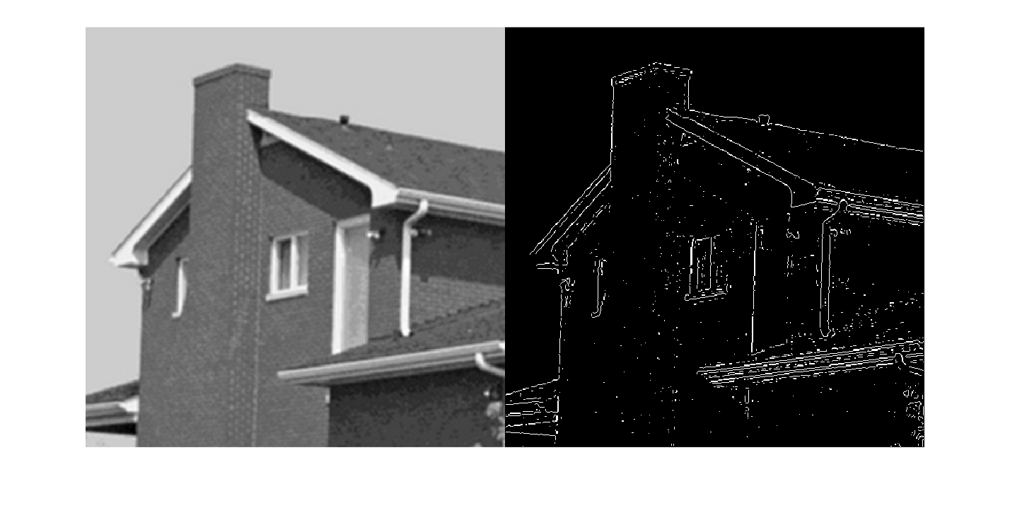
The Marr-Hildreth method combines smoothing and detection of intensity changes. First, noise is reduced with a Gaussian filter, and then the Laplacian is applied. Edges are located by searching for zero crossings, that is, points where the response changes sign. This idea can detect important transitions, but the result depends on the smoothing scale and the selected threshold.

house = imread("Imagenes\house.tif");
house = house(:,:,1);
w_log = fspecial("log",25,1);

T = 0.018 (empirical, that is, calculated by trial and error).

The threshold controls which responses are considered strong enough to belong to an edge. If it is too low, many false edges appear; if it is too high, real contours may be lost. This is why it is often adjusted empirically by observing the result.

T = 0.018;

edge is used for MH with the zerocross option, adding the threshold T and the kernel of a filter, in this case a Laplacian of Gaussian (LoG) filter.

house_contornos = edge(house,"zerocross",T,w_log);

montage({house,house_contornos})

Canny method

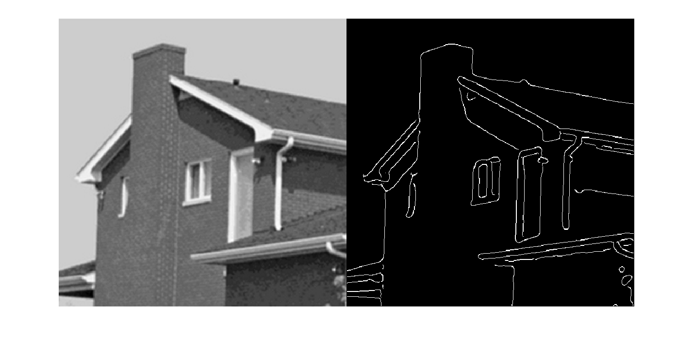
The Canny detector is a more complete edge-detection method. It includes initial smoothing, gradient computation, selection of local maxima and a final decision with two thresholds. The high threshold identifies strong edges, while the low threshold preserves weak edges if they are connected to strong ones. This helps obtain cleaner and more continuous contours.

We define the lower and upper thresholds (also calculated empirically).

T_canny = [0.04,0.2];

The edge command is used to apply the Canny method (with the "canny" option). As extra inputs, a threshold must be added (in this case a vector of two thresholds, lower and upper) and the variance of the first step, which is used to smooth the image with a Gaussian filter.

sigma = 4;

house_canny = edge(house,"canny",T_canny,sigma);

montage({house,house_canny})

We experiment with the lower and upper thresholds (Important! T1 must always be less than T2 and T2<1)

T1 = 0.01:0.03:0.07;
T2 = 0.1:0.2:0.9;
sigma = 4;

% for i = 1:length(T1)
% 
%     for j = 1:length(T2)
% 
%         if T1(i)<T2(j)
% 
%             house_canny_loop = edge(house,"canny",[T1(i),T2(j)],sigma);
% 
%             figure;
%             imshow(house_canny_loop)
% 
%         end
% 
%     end
%
% end

Segmentation methods based on similarity

Similarity-based methods start from a different idea: pixels in the same region should share some property. This property may be intensity, color, texture or spatial proximity. Instead of only searching for boundaries between regions, these methods try to build coherent regions from the inside.

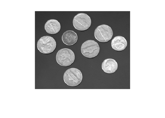
We load the image that we will use.

monedas = imread("Imagenes\coins.png");

imshow(monedas)

Watershed --> Segmentation method based on a basin flooding process, that is, from the different minima of the image, and on the construction of dams, that is, edges, separating the different regions.

An intuitive way to understand watershed is to imagine the image as a topographic surface. Minimum regions are filled as if they were water basins, and when two basins meet, a boundary is built. These boundaries become the separation lines between regions.

monedas_watershed = watershed(monedas);

We keep the separation lines (which are black) in the output of the watershed command. That is, "bordes" is a binary image that has all the black pixels of the output, "monedas_watershed", which are precisely those separation lines, as pixels with intensity value 1, that is, white.

bordes = monedas_watershed == 0;

We merge it with the original image and convert the separation lines into white lines so that they stand out when they are superimposed on the original image. First we make a copy of the original image so as not to alter it.

monedas_copia = monedas;

And then we change the pixels that in the binary image "bordes" do not belong to the image background to white pixels, that is, with intensity level 255.

monedas_copia(bordes) = 255;

Finally, we display the result.

montage({monedas,monedas_copia})

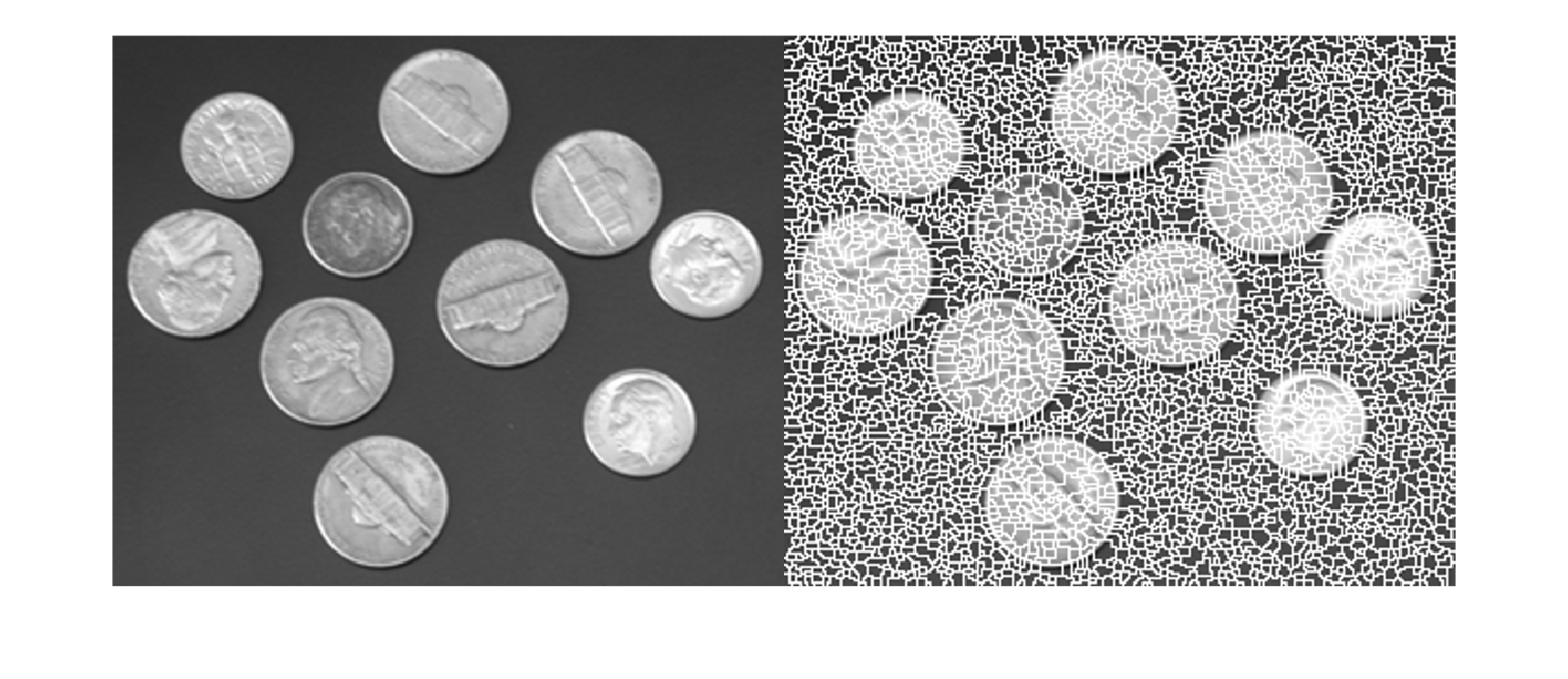
There is clearly oversegmentation, so we try different ways to solve this oversegmentation.

Oversegmentation occurs when a method divides a region that visually corresponds to a single object into many small parts. In watershed segmentation, this often happens because the image contains many local minima, some of which are caused by noise or small intensity variations. To improve the result, irrelevant minima must be reduced or more reliable markers must be imposed.

1st method --> connectivity option. The "watershed" command accepts a second input, which is the connectivity of the original image. This connectivity can improve the result by removing the dams associated with connected components that are not compatible with the imposed connectivity.

Connectivity defines which pixels are considered neighbors. In a 2D image, a more restrictive connectivity can separate regions that only touch diagonally, while a more permissive one can consider them connected. This decision directly affects the final watershed regions.

monedas_watershed_2 = watershed(monedas,8);

bordes_2 = monedas_watershed_2 == 0;

monedas_copia_2 = monedas;

monedas_copia_2(bordes_2) = 255;

montage({monedas_copia_2})

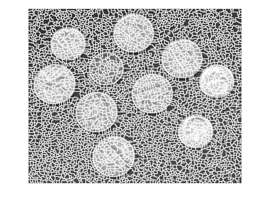
2nd method --> use of the distance transform. The distance transform allows the geometric center of the objects to be found (not of the connected components, but of the objects (two objects touching each other can form a single connected component)). In fact, this is one of the great advantages of watershed, which allows images with touching or partially overlapping objects to be segmented.

In binary objects, the maxima of the distance transform are usually close to the center of each object. If this information is used as a basis for watershed, touching objects with different centers can be separated. This strategy is very common in images containing coins, cells or particles.

To apply the distance transform, we need a binary image. To do this, we binarize using Otsu's method.

T_otsu_monedas = graythresh(monedas);

monedas_bin = imbinarize(monedas,T_otsu_monedas);

We calculate the distance transform.

D = bwdist(monedas_bin);

We apply the watershed algorithm to the result.

D_watershed = watershed(D);

bordes_D = D_watershed == 0;

monedas_copia_3 = monedas;

monedas_copia_3(bordes_D) = 255;

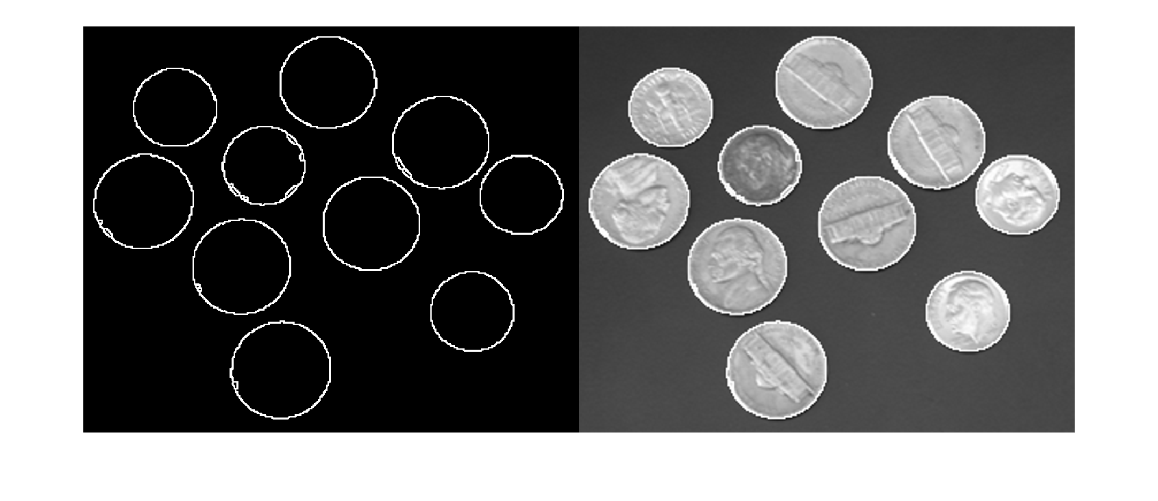
montage(monedas_copia_3)

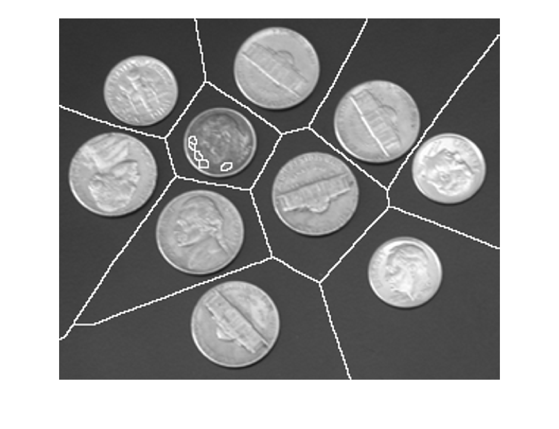
3rd method --> use of the gradient. The gradient magnitude of the image allows ALL the minima of the image to be detected (the real ones and those that produce oversegmentation).

When watershed is applied on the gradient, strong edges act as natural barriers between regions. The problem is that the gradient may also contain small minima caused by noise or texture. This is why minima are filtered or imposed afterwards, to guide the segmentation more reliably.

w_sobel = fspecial("sobel");

gradient_mag = abs(imfilter(double(monedas),w_sobel))+abs(imfilter(double(monedas),w_sobel'));

We filter the minima so that only the deepest ones survive. The "imextendedmin" command takes an image of regional minima (like the one returned by the gradient) and removes all pixels with an intensity value greater than the second input. The output of the command is a binary image with the deepest minima.

minimos = imextendedmin(gradient_mag, 200);

We force the gradient minima to be only those that survive the previous command. To do this, the "imimposemin" command is used, which imposes on the first input a set of minima, which is the second input.

minimos_forzados = imimposemin(gradient_mag, minimos);

monedas_watershed_3 = watershed(minimos_forzados);

bordes_3 = monedas_watershed_3 == 0;

monedas_copia_3 = monedas;

monedas_copia_3(bordes_3) = 255;

montage({bordes_3,monedas_copia_3})