Tutorial and exercises

Mathematical morphology studies images through the shape of objects. In binary images, white pixels can naturally be interpreted as the object set and black pixels as the background. Morphological operations modify this set using a small shape, called a structuring element, which acts as a geometric probing tool.

The structuring element is an essential part of the method. Its size determines the scale of details that are removed or preserved, and its shape determines which structures fit the operation better. Choosing a disk, a line, a square or another shape is therefore not only a technical decision, but a way of expressing what type of geometry should be analyzed.

We load the binary images that we will use during the practical session

figuras = imread("Imagenes\figures.png");
head = imread("Imagenes\head.png");
agujeros = imread("Imagenes\agujeros.png");
simbolos = imread("Imagenes\Simbols.jpg");
scissors = imread("Imagenes\scissors.tif");

We transform all images that are not binary into binary images

In this practical, the usual convention is used: objects are white and the background is black. This convention matters because morphological operations act on foreground pixels. If the image is inverted, an operation expected to grow an object may end up affecting the background, and the interpretation of the result changes.

figuras = rgb2gray(figuras);
figuras = figuras<128;

agujeros = agujeros>128;

simbolos = rgb2gray(simbolos);
simbolos = imresize(simbolos,[512,512]);
simbolos = simbolos<128;

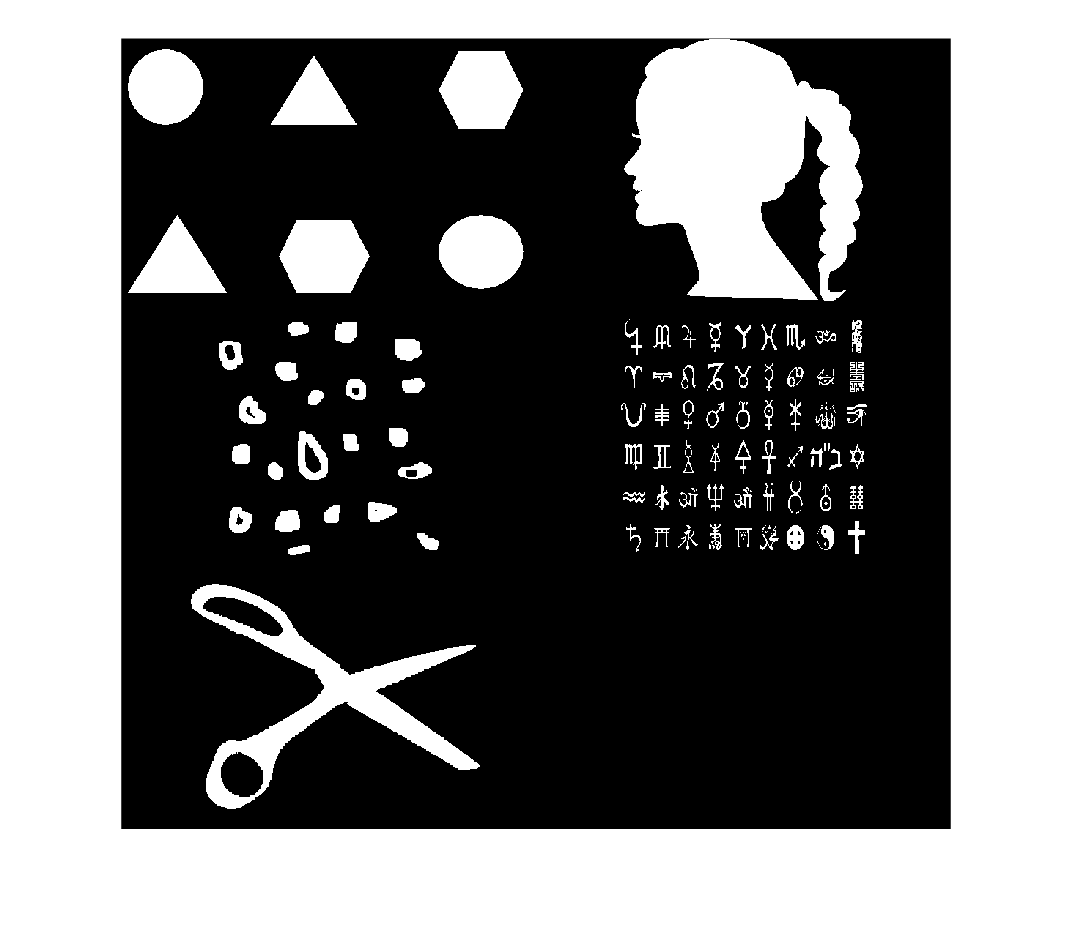
montage({figuras,head,agujeros,simbolos,scissors})

Primary morphological operators

The primary operators are dilation and erosion. Dilation grows white regions and can join nearby parts of an object. Erosion has the opposite effect: it reduces white regions and removes small parts where the structuring element cannot fit completely. These two operators are the basis of many more complex morphological operations.

Definition of structuring elements. The strel command is used, whose input is the type of structuring element, which can be a disk, diamond, line, rectangle, square, and shapes defined by matrices.

The structuring element defines which neighbors are considered in each morphological operation. A disk treats directions more uniformly, a line emphasizes one specific orientation, and a square considers a compact neighborhood. Therefore, before applying the operation, it is important to think about the shape of the detail that should be preserved or removed.

SE = strel("diamond",1);

Types of structuring elements and their parameters:

• diamond -- distance from the origin to the end of the diamond (1 for cross)
• disk -- radius
• line -- length and angle
• rectangle -- length and height (enter as a vector, that is, \(begin:math:display\)l\,a\(end:math:display\))
• square -- side
• nhood -- shape defined by a matrix of 0s and 1s

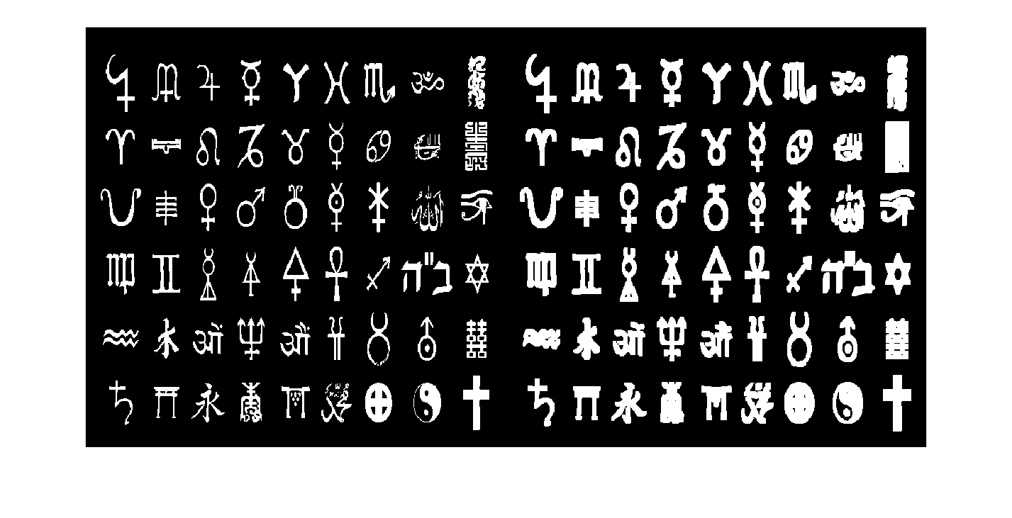
Dilation. The imdilate command is used, whose input is the binary image to be dilated and the structuring element by which it is dilated. Try diamond 1, square 3, disk 10.

When the structuring element changes, the way the object grows also changes. A small element only modifies the contour slightly, while a large disk may join nearby regions and remove narrow gaps. This experiment shows that morphology strongly depends on the chosen scale.

SE = strel("square",4);

%SE = strel("disk",10);

scissor_dilate = imdilate(scissors,SE);

montage({scissors,scissor_dilate})

simbolos_dilate = imdilate(simbolos,SE);

The effect will be the expected one, that is, dilating the objects in the image.

montage({simbolos,simbolos_dilate})

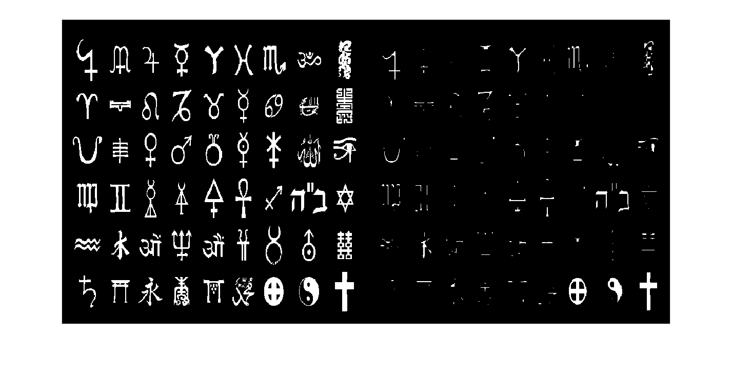
Erosion. The imerode command is used, whose input is the binary image to be eroded and the structuring element by which it is eroded.

Erosion removes contour pixels when the structuring element does not fit completely. It can therefore separate objects connected by narrow bridges or remove small components. It can also remove useful details if the structuring element is too large.

simbolos_erode = imerode(simbolos,SE);

The effect is the expected one: the objects in the image are reduced.

montage({simbolos,simbolos_erode})

Edge extraction in binary images.

In binary images, an edge can be obtained by comparing the original object with an eroded or dilated version of it. This idea is different from gradient-based edge detection, because here the method does not measure intensity changes; it measures changes in the shape of the set of white pixels. This makes morphological edges especially appropriate when the image has already been segmented.

Method 1: image-erosion(image)

head_erode = imerode(head,SE);

head_bordes = head-head_erode;

montage({head,head_bordes})

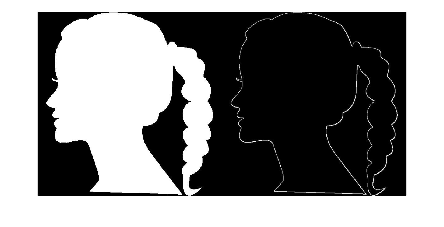
This is considered an inner edge (which comes from an inner residue, which is always generated from erosion by a structuring element).

Outer edge (outer residue, which is always generated from dilation by a structuring element).

head_dilate = imdilate(head,SE);

Since the dilation of an image is always larger than the image (remember that, in fact, it contains the image), instead of doing image -dilation(image), we have to do dilation(image)-image.

head_bordes_2 = head_dilate-head;

We compare the two types of edges. Pay attention to the small details (such as the eyelashes and lips) to understand why one is called an inner edge and the other an outer edge.

montage({head_bordes,head_bordes_2})

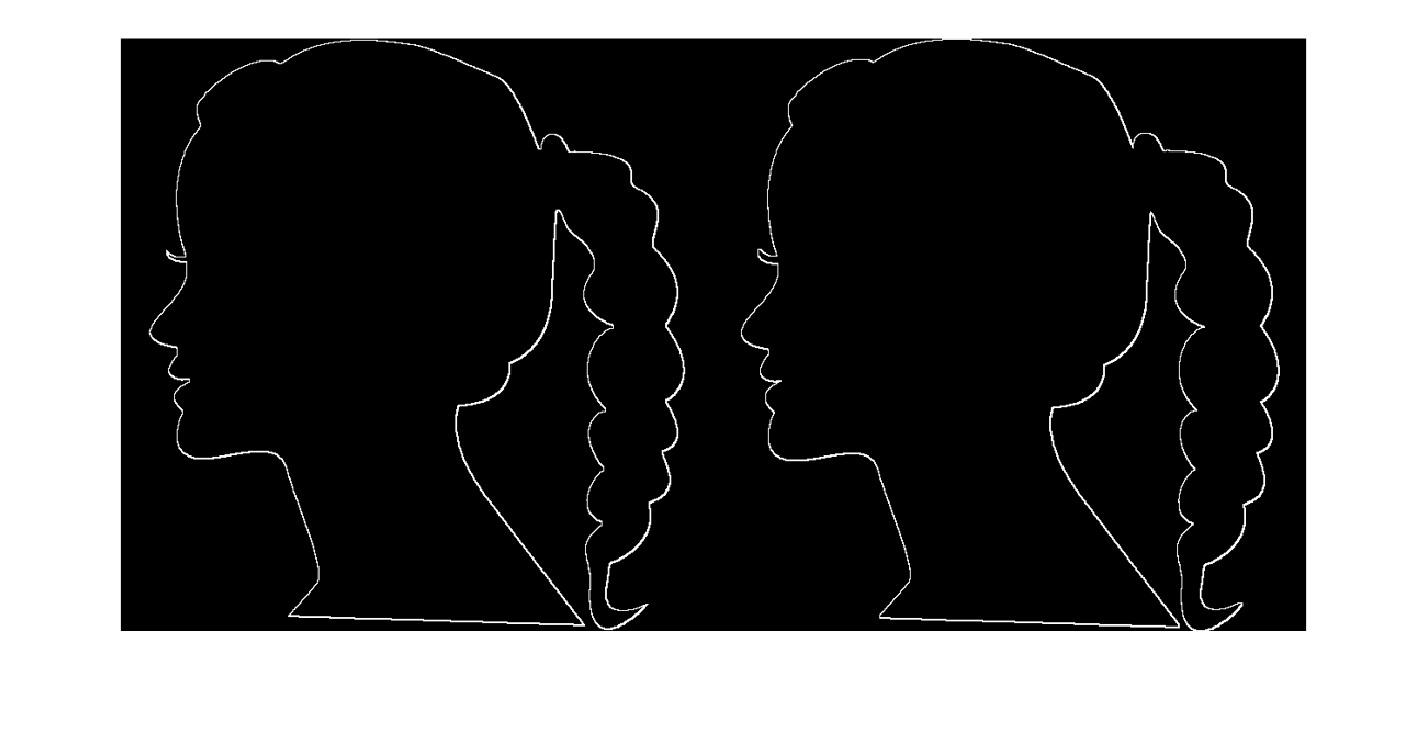
Internal-external residue (that is, both together). It is produced by subtracting the erosion of the image from the dilation of the image.

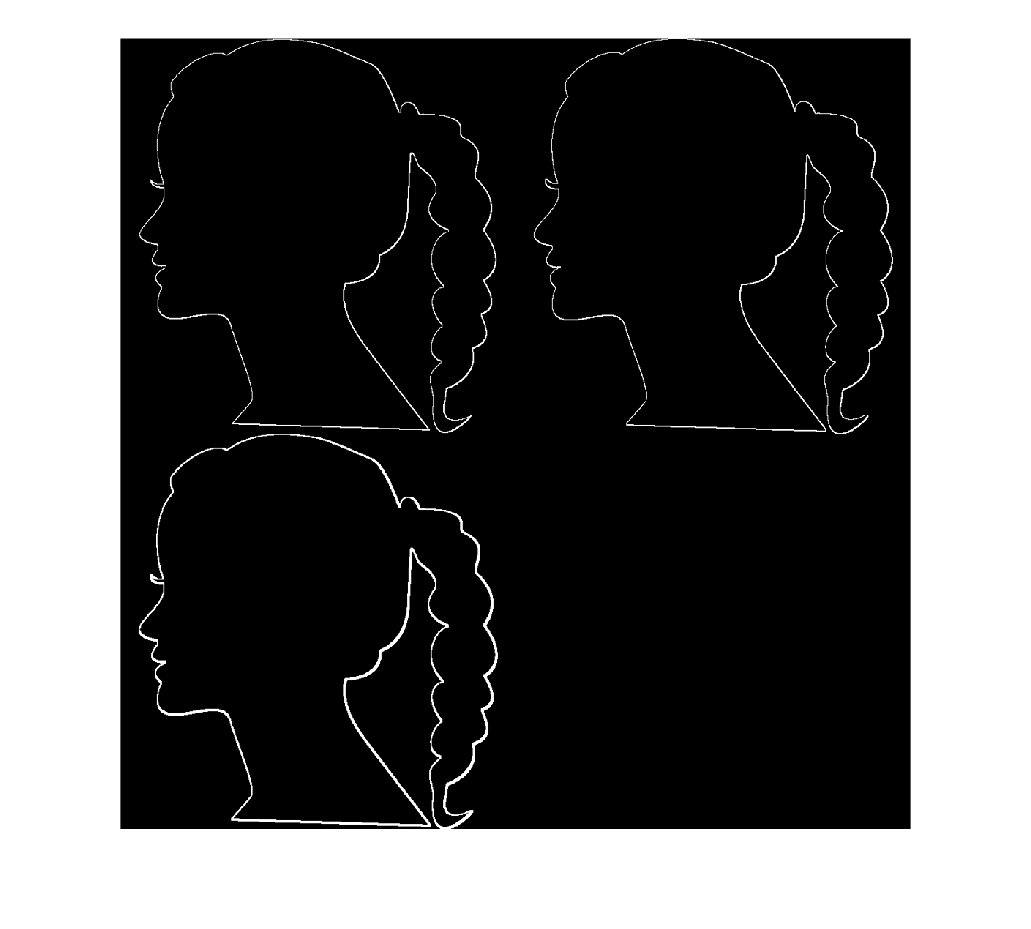
head_bordes_3 = head_dilate-head_erode;

Notice that this edge is always thicker than the inner or outer edge. This is because this edge contains the inner and outer edges, since it has been calculated with both residues.

montage({head_bordes,head_bordes_2,head_bordes_3})

Filling holes and interiors. The imfill command is used, where the input is the image with holes. The "holes" option must be added.

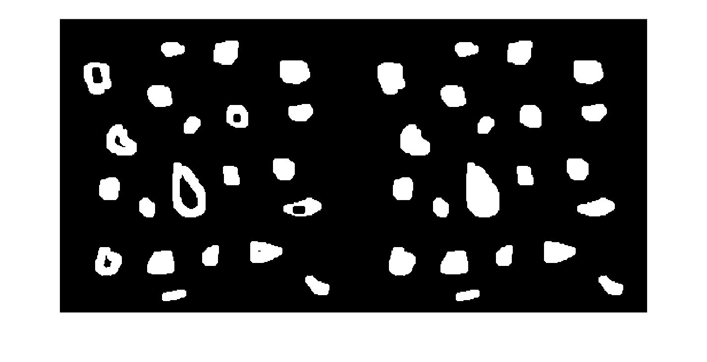
A hole is a background region completely surrounded by object pixels. Filling holes is useful when segmentation has left internal gaps that are not really part of the background. This operation preserves the outer contour but changes the internal topology of the object.

agujeros_fill = imfill(agujeros,"holes");
montage({agujeros,agujeros_fill})

Reconstruction of connected components by dilation.

Morphological reconstruction can be understood as controlled growth. It starts from a marker, which indicates which pixels are known to belong to the object to be recovered, and a mask, which limits growth to the allowed regions. In this way, specific connected components can be reconstructed without modifying the rest of the image.

Uncomment this part when you get here. This command displays the image in an independent window so that you can click on one of the symbols, which will be the one we reconstruct.

% imshow(simbolos)

This command keeps the coordinates (in double) of the point marked with the mouse in the simbolos image. We have to select a point to reconstruct the connected component associated with that point.

%[x,y] = getpts;

Binary image of zeros. The false command creates a binary image of the size of the input. In this image, in this case of the same size as the original image, we will only change the value of one pixel, which will be the value of the pixel marked with the mouse using the getspts command.

%pointer = false(size(simbolos));

We assign the selected point and turn it white. Remember that to reconstruct connected components, the algorithm started with a point that we know belongs to the connected component. In this case, it will be the point marked with the mouse.

%pointer(uint16(y),uint16(x)) = 1;

The uint16 command only converts x and y into integers, so that we know which pixel is the marker. We do not use uint8 because the marker is on a scale greater than 255 (because the getspts command can be used with images of any type, in particular, high-intensity images). We reconstruct the connected object to which the selected point belongs. To do this, the imreconstruct command is used, whose parameters are the image with the point or points of the connected components to be reconstructed and the original image that will serve as the pattern in the reconstruction.

%simbolos_recons = imreconstruct(pointer,simbolos);

If you click on more than one symbol with the mouse, imreconstruct will reconstruct all of them.

%montage({simbolos,simbolos_recons});

Secondary morphological operators

Opening and closing are secondary operations because they combine erosion and dilation. Opening first erodes and then dilates, so it tends to remove small objects or thin protrusions. Closing first dilates and then erodes, so it tends to fill small holes, close narrow gaps and smooth indentations in the contour.

Opening. The opening operator is applied using the imopen command. This command has as parameters the image to be opened and the structuring element that will be used.

SE = strel("disk",5);

figures_open = imopen(figuras,SE);

Notice that the outer corners of the triangle and the pentagon are now rounded instead of pointed. This is one of the typical effects of applying the opening operator.

montage({figuras,figures_open})

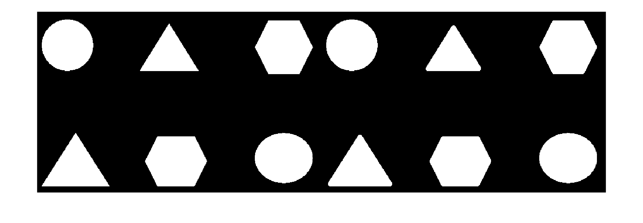
Closing. Like the opening operator, this operator is applied using the imclose command, which has the same inputs as the opening operator.

figures_close = imclose(figuras,SE);

Notice that in this case no changes are observed in the image. This is because the closing operator rounds inner corners, which are not present in this case. Let us look for another example.

montage({figuras,figures_close})

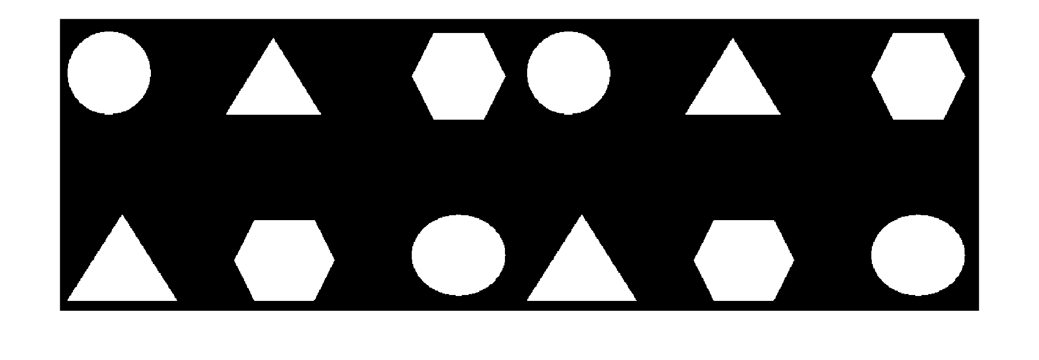
scissors_close = imclose(scissors,SE);

Notice that in this case, the inner corners of the object appear rounded instead of pointed, which is a typical effect of the closing operator.

montage({scissors,scissors_close})

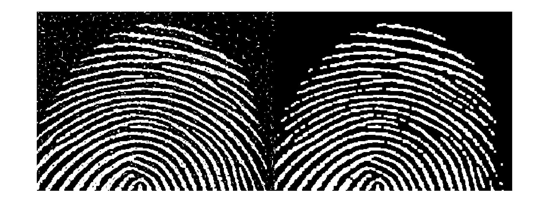
Morphological filtering. It is a "smoothing" filter but based on morphological operators. In particular, it is very good with salt and/or pepper noise.

Morphological filtering does not average pixel values; it uses shape operations. This is useful when noise appears as small white or black dots, because these dots can disappear if they are smaller than the structuring element. At the same time, large and coherent structures can be preserved better than with linear smoothing.

Remember --> Filtering = Closing of the opening of the image

Applying an opening first helps remove small white points or thin protrusions. Applying a closing afterwards helps recover continuity and fill small gaps. The combination is useful as a morphological filter because it removes small noise without relying on intensity averaging.

huellas = imread("Imagenes\Huella.jpg");

We binarize the Huella image

huellas = rgb2gray(huellas);
huellas = huellas>128;

SE = strel('square',5);

huellas_open = imopen(huellas,SE);

huellas_filt = imclose(huellas_open,SE);

montage({huellas,huellas_filt})

Hit-or-miss transform and reconstruction by dilation. The hit-or-miss transform takes a structuring element that is equal to the connected component that you want to find in the original image, and returns a point of the component, to then reconstruct it as we have seen before. It is a way of automatically detecting points of the connected components that we want to reconstruct, without having to click with the mouse.

The hit-or-miss transform searches for a specific configuration in a binary image. One part of the pattern must match object pixels and another part must match background pixels. It is therefore useful for detecting very specific shapes, although it may fail if the object is deformed, rotated or affected by noise.

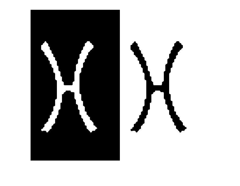
We take a structuring element that has the shape of one of the symbols in the image.

SE1 = simbolos(25:110,285:335);

montage({simbolos,SE1})

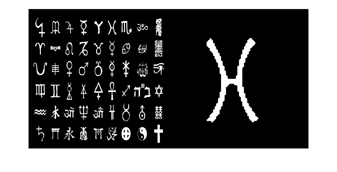
Remember that the second structuring element must be the complement of the first one.

SE2 = not(SE1);

montage({SE1,SE2})

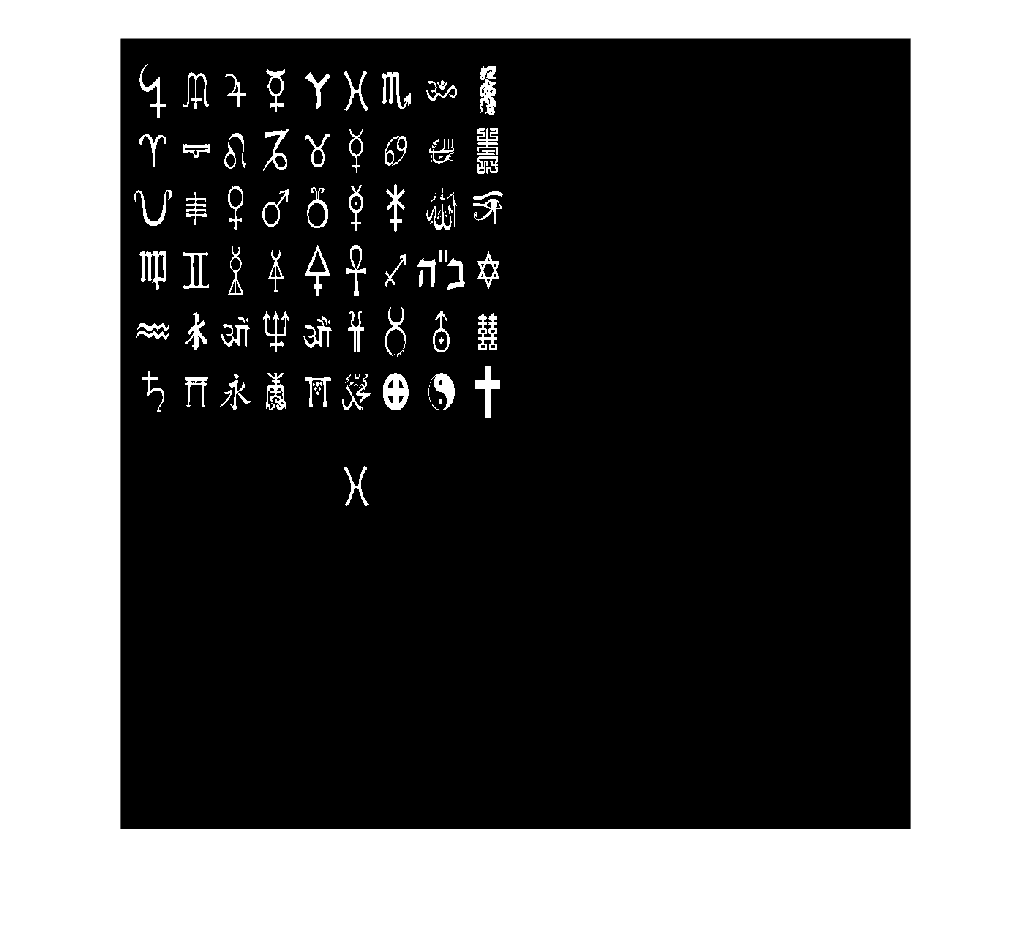
The hit-or-miss transform is applied with the bwhitmis command, whose inputs are the original image and the two structuring elements.

pointer = bwhitmiss(simbolos,SE1,SE2);

Once the point of the connected component to be reconstructed has been obtained, we reconstruct it as we have seen before.

simbolos_re=imreconstruct(pointer,simbolos);

montage({simbolos,pointer,simbolos_re})

Skeletonization. One of the applications of the hit-or-miss transform is to calculate the skeleton of the elements in a binary image. There are mainly two ways.

Skeletonization tries to reduce an object to a thin structure, ideally one pixel wide, while preserving its main connectivity. This representation is useful for studying elongated shapes, branches or geometric centers. However, if the contour is irregular or noisy, small undesired branches, called spurious elements, may appear.

1st method, using the bwskel command, whose input is the original image.

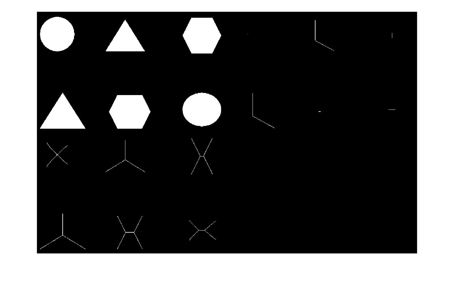
figures_sk = bwskel(figuras);

2nd method, using the bwmorph command, whose inputs are the original image, "skel" to indicate that the morphological transformation we want to perform is to obtain the skeleton, and Inf, which prunes spurious elements (that is, branches of the skeleton that should not be there).

figures_ske = bwmorph(figuras,'skel',Inf);

We compare both methods. Although it may seem that bwmorph produces a better result, in general, the best way to calculate the skeleton is with bwskel. Let us see other examples.

montage({figuras,figures_sk,figures_ske})

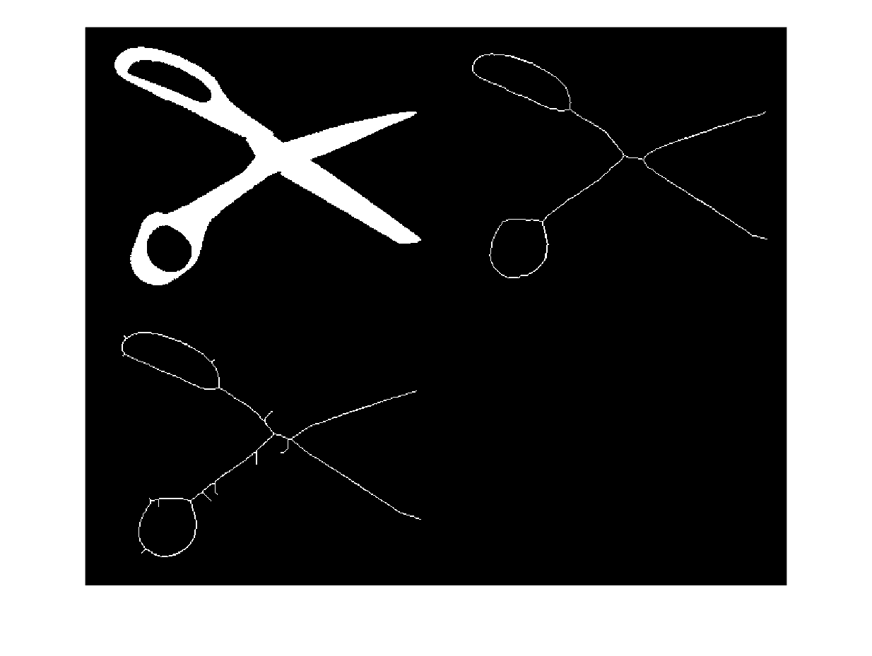
scissors_sk = bwskel(scissors);

scissors_ske = bwmorph(scissors,'skel',Inf);

Here we can observe that bwmorph produces a worse result (and with spurious elements despite the Inf command).

montage({scissors,scissors_sk,scissors_ske})

head_sk = bwskel(head);

head_ske = bwmorph(head,'skel',Inf);

Same comment as before.

montage({head,head_sk,head_ske})

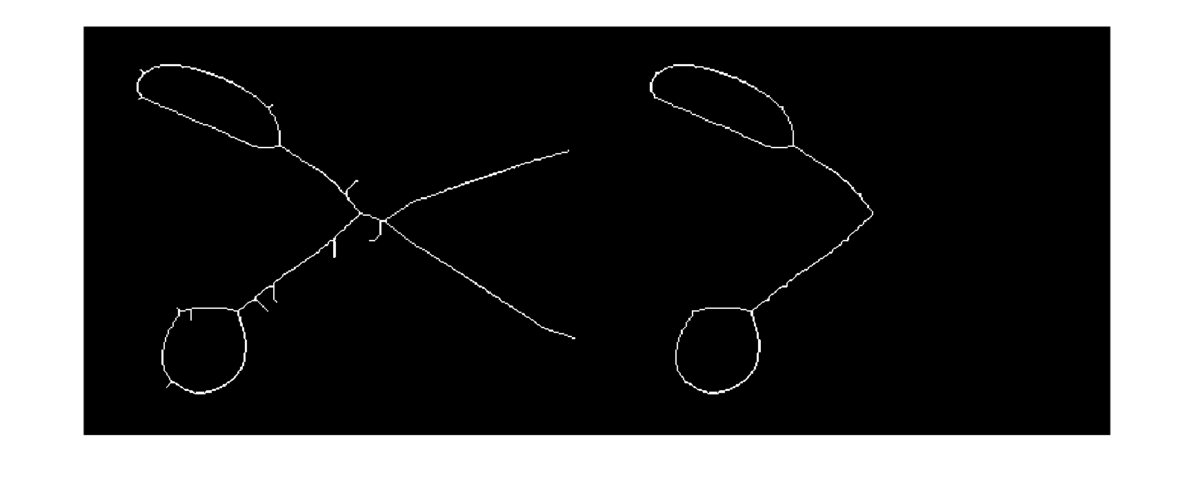
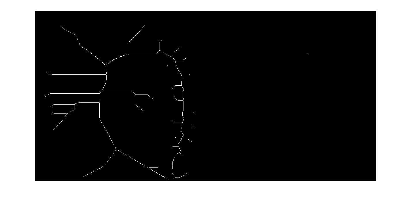
In cases like the previous ones where bwmorph shows a skeleton with undesirable (spurious) elements, there is a command to prune the skeleton even more. It is again bwmorph. In this case, the only thing that changes is that instead of asking for "skel" so that it makes the skeleton, we ask for "spur" so that it prunes spurious elements.

scissors_poda = bwmorph(scissors_ske,"spur",Inf);
head_poda = bwmorph(head_ske,"spur",Inf);

In both cases the result is still poor, which confirms that the bwskel option is the best.

montage({scissors_ske,scissors_poda})

montage({head_ske,head_poda})

Skeleton calculation can also be used to segment the image (if it is binary). To do this, the first step is to apply not() to the image, since the skeleton is always calculated in the area with pixels of value one (white here).

figuras = not(figuras);

agujero = not(agujeros_fill);

montage({figuras,agujero})

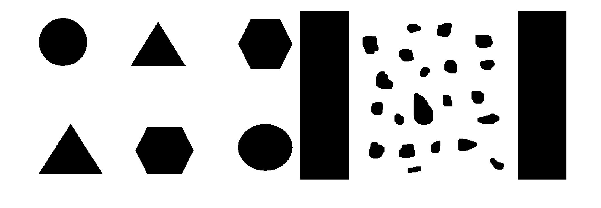
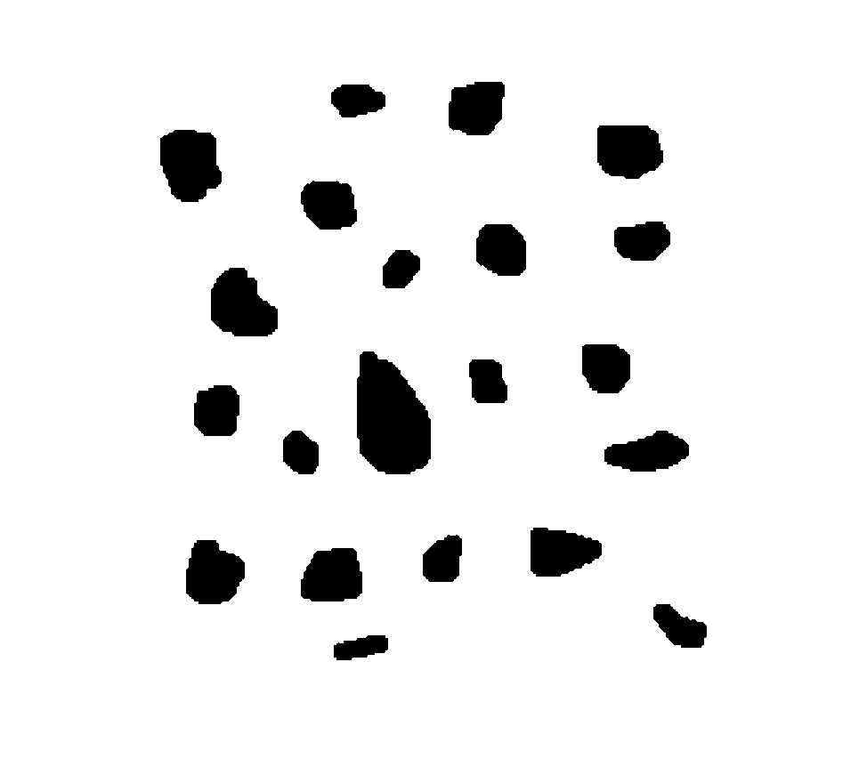
Since the agujero image has two black strips around it, we use a small trick. This consists of defining a white frame around the image and applying the closing operator. This will automatically turn all the background that was not yet white into white.

Command to make the outer border of the image white.

agujero(1,:)=1; agujero(end,:)=1; agujero(:,1)=1; agujero(:,end)=1;

agujero = imclose(agujero,SE);

Result.

montage(agujero)

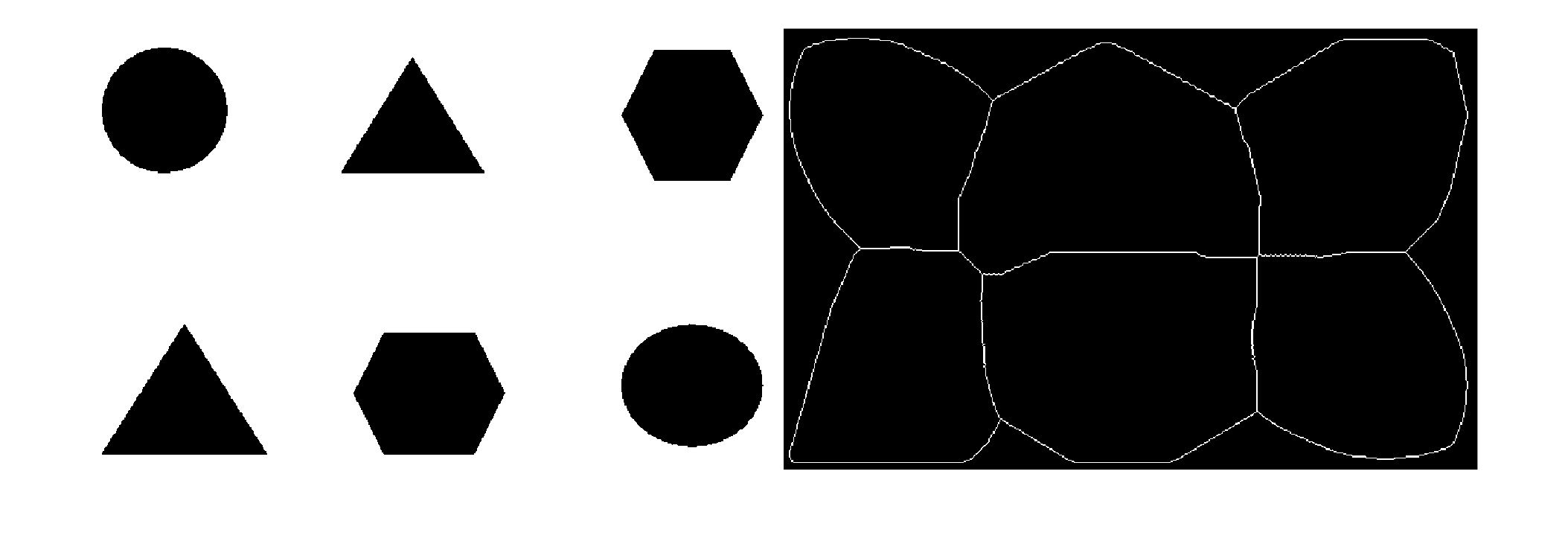
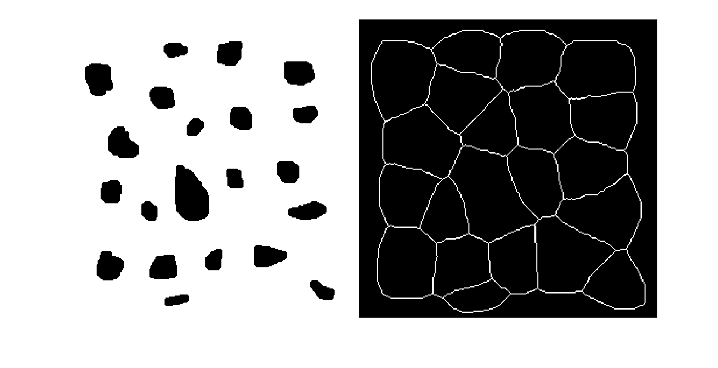
Now, we skeletonize with bwskel and see that it has delimited the areas where each of the figures or each of the objects is located, which is in fact segmenting the image into different areas according to the objects.

figuras_sk = bwskel(figuras);

agujero_sk = bwskel(agujero);

montage({figuras,figuras_sk})

montage({agujero,agujero_sk})

bwmorph can also be used to perform all the other operations we have seen before (dilation, erosion, opening, etc.) but only with 3x3 square structuring elements, so in practice it is not used.

If now we wanted to segment a binary image with elements on the border, such as the one shown below, we would discover that the segmentation does not work. A trick to fix this problem consists of removing the border elements.

test_morph = imread("Morfologia_I.jpg");

test_morph = rgb2gray(test_morph);
test_morph = test_morph > 128;

montage(test_morph)

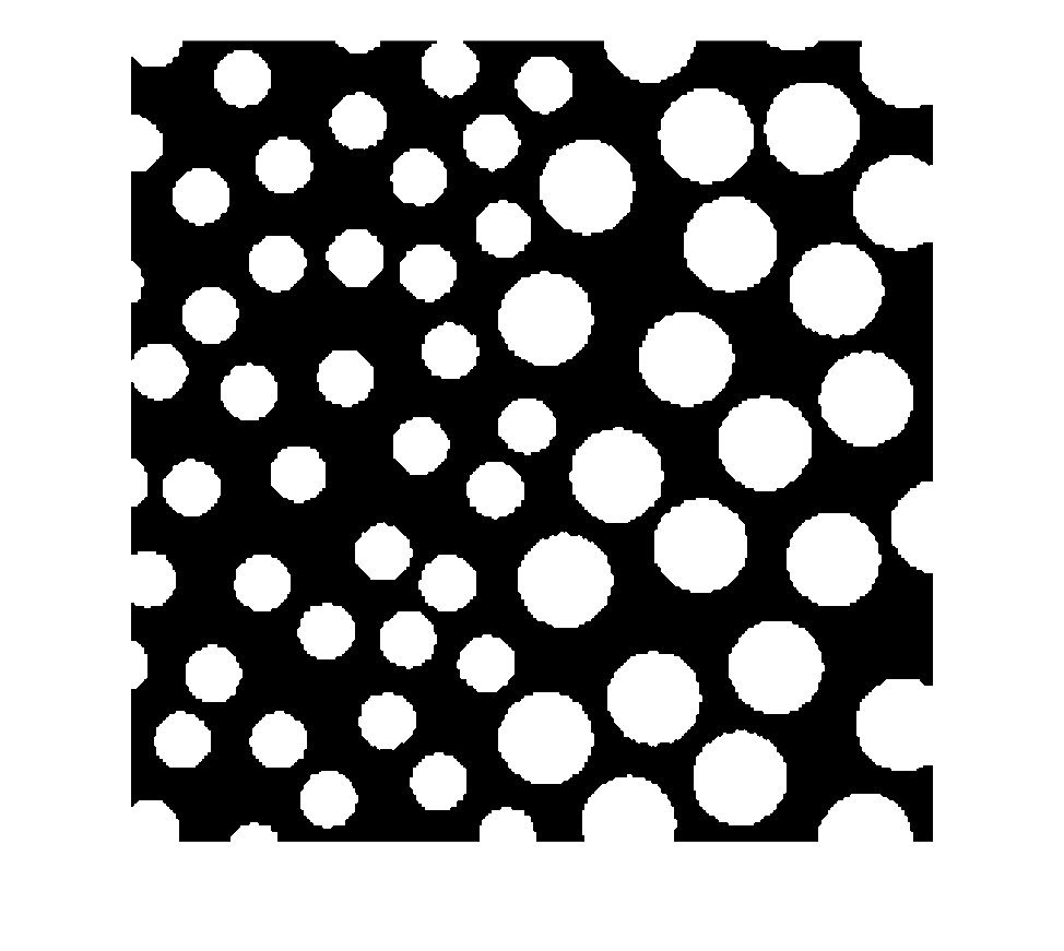
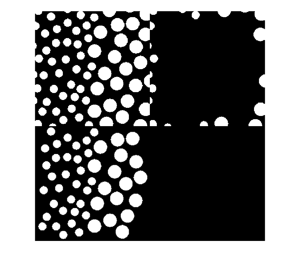
To do this, we are going to create a binary image that will only have white values on the border and reconstruct it based on the original image. This will give us the border elements, which we simply have to subtract from the original image.

pointer = false(size(test_morph));

We define white borders

pointer(1,:)=1; pointer(:,1)=1; pointer(end,:)=1; pointer(:,end)=1;

We reconstruct

test_morph_recon = imreconstruct(pointer,test_morph);

We subtract to keep the interior elements.

test_morph_no_bordes = test_morph - test_morph_recon;

montage({test_morph,test_morph_recon,test_morph_no_bordes})

Distance transform

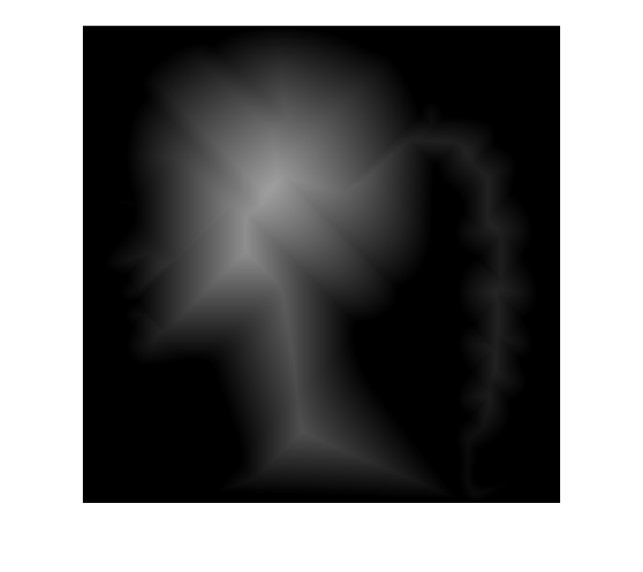
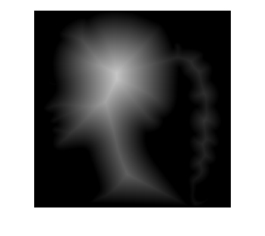
The distance transform assigns each object pixel a value related to its distance to the nearest background pixel. The result is no longer a binary image, but a grayscale image that describes the interior of the shapes. The highest values usually appear near object centers, which is useful for computing skeletons or separating touching objects.

Distance transform. This calculates the distance to the nearest border of each white element in the original image. In this way, we convert the binary image into a grayscale image. The element furthest from the borders will be 255, and so on proportionally as we get closer to the borders.

Since we want to apply it to the silhouette, we have to convert the silhouette to white and the background to black.

head_neg = not(head);

imshow(head_neg)

The distance transform is applied with the bwdist command, where the only input is the original image to be transformed.

head_d = bwdist(head_neg);

To view the images, we need to add \(begin:math:display\)\(end:math:display\)

imshow(uint8(head_d))

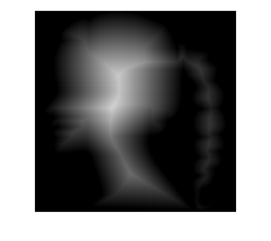
Other distances (cityblock -- Manhattan or d4, chessboard -- chessboard or d8).

Euclidean distance measures the usual geometric distance, while cityblock allows only horizontal and vertical moves, and chessboard also allows diagonal moves with the same cost. Changing the metric modifies the shape of the distance levels and can therefore affect skeletons or estimated centers.

head_d4 = bwdist(head_neg,"cityblock");
head_d8 = bwdist(head_neg,"chessboard");
imshow(uint8(head_d4))

imshow(uint8(head_d8))