Tutorial and exercises

This practical focuses on local features that make it possible to find correspondences between images. A correspondence means that a point in one image and a point in another probably represent the same part of the scene or the same object. For this to work, the detector must find repeatable points and the descriptor must represent them in a stable enough way under changes in scale, rotation, viewpoint or illumination.

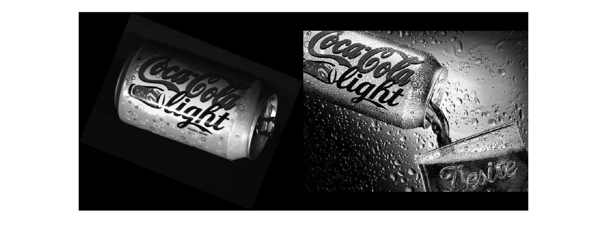
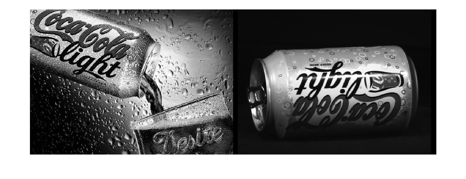
We load the images that we will use in the practical session

cocacola_lata_1 = imread("Imagenes\coca_cola_1.jpg");
cocacola_lata_2 = imread("Imagenes\coca_cola_2.jpg");
frame1 = imread("Imagenes\Frame 1.tif");

We convert the images to grayscale (for better feature detection)

Many local detectors work on intensity because corners, edges and gradients can be clearly defined in a single grayscale image. This reduces complexity and prevents less relevant color differences from interfering with detection.

cocacola_lata_1 = rgb2gray(cocacola_lata_1);
cocacola_lata_2 = rgb2gray(cocacola_lata_2);

montage({cocacola_lata_1,cocacola_lata_2})

SIFT-type features

SIFT is designed to detect stable interest points. One of its main ideas is to analyze the image at different scales, because the same object may appear larger or smaller depending on its distance from the camera. It also assigns an orientation to detected points and computes gradient-based descriptors, which helps compare points even when the image is rotated or has moderate illumination changes.

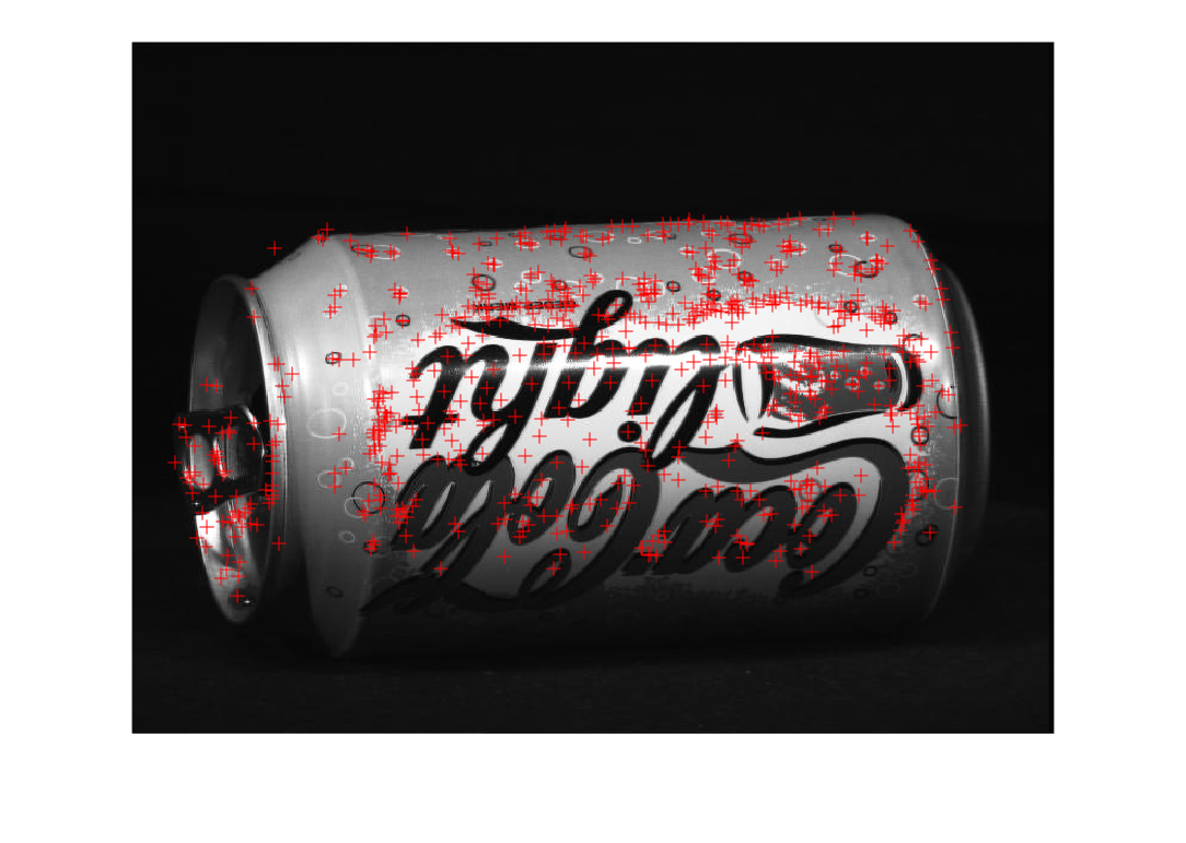
We use the detectSIFTFeatures command to obtain all SIFT-type interest points together with their descriptors. Then we display them over the original image to see what type of features this algorithm detects.

SIFT_features_lata_2 = detectSIFTFeatures(cocacola_lata_2);
puntos_SIFT_lata_2 = SIFT_features_lata_2.Location;

imshow(cocacola_lata_2)
hold on
plot(puntos_SIFT_lata_2(:,1),puntos_SIFT_lata_2(:,2),'+',Color='r');
hold off

Analysis of the input parameters: threshold for the maxima and minima, that is, for non-maximum suppression, threshold to remove interest points belonging to lines, definition of the number of layers in the octaves and of the initial value of the variance.

Detector parameters directly influence the number and quality of detected points. If thresholds are too permissive, many points appear, but some may be unstable or correspond to noise. If thresholds are too strict, the number of points decreases and useful regions may be lost. These parameters should therefore be understood as a balance between sensitivity and reliability.

Another example

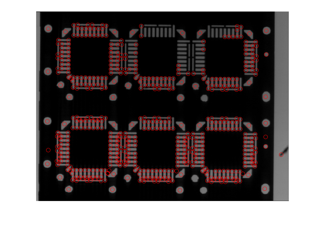
SIFT_features_frame_1 = detectSIFTFeatures(frame1);

puntos_SIFT_frame_1 = SIFT_features_frame_1.selectStrongest(550);

puntos_SIFT_frame_1 = puntos_SIFT_frame_1.Location;

imshow(frame1);
hold on
plot(puntos_SIFT_frame_1(:,1),puntos_SIFT_frame_1(:,2),'o',Color='r')
hold off

FAST-type features

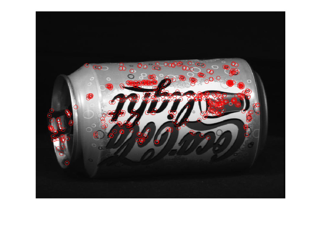
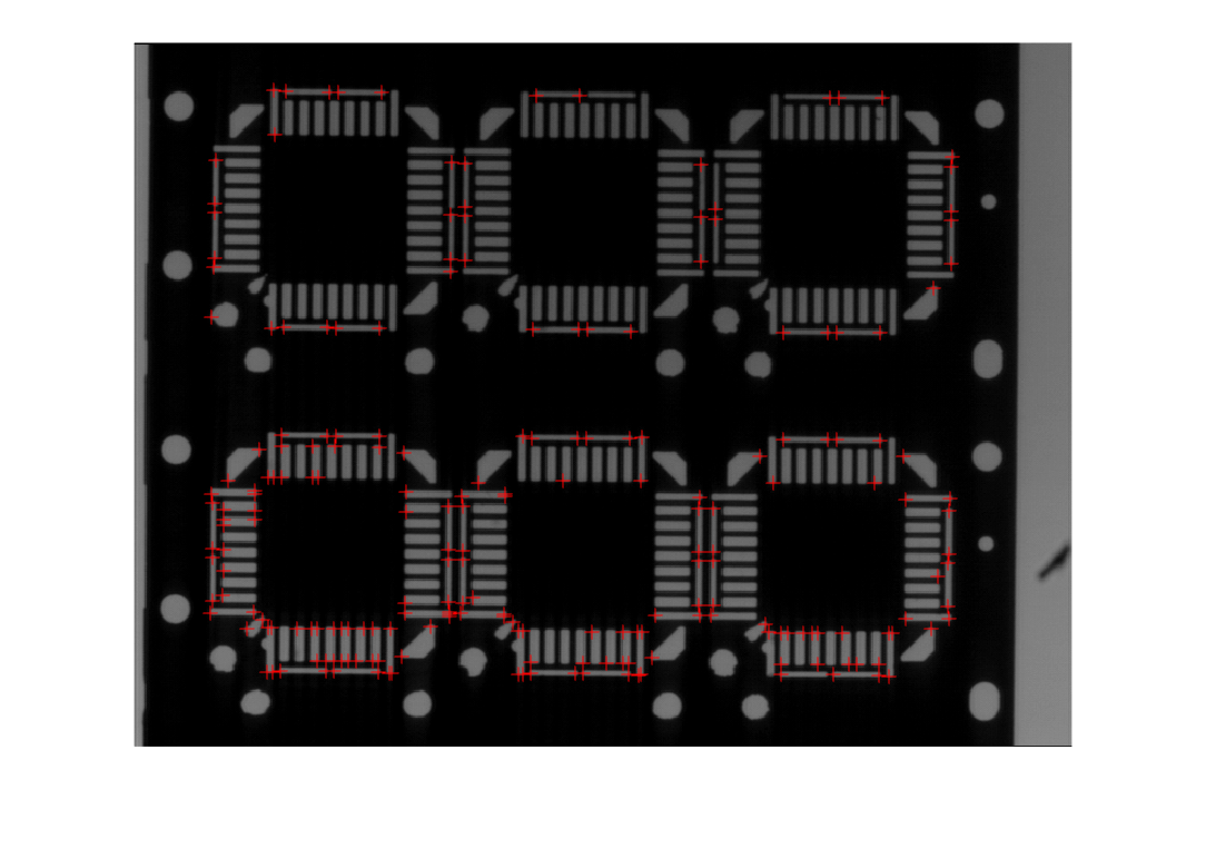
FAST is a corner detector designed to be very fast. It analyzes pixels on a circle around the candidate point and checks whether there is a sufficiently clear intensity change. This simplicity makes it very efficient in applications where computation time matters. However, FAST detects points but does not by itself provide a complete descriptor for comparing them across images.

We use the detectFASTFeatures command to obtain all FAST-type interest points. Then we display them over the original image to see what type of features this algorithm detects.

FAST_features_lata_2 = detectFASTFeatures(cocacola_lata_2);

puntos_FAST_lata_2 = FAST_features_lata_2.Location;

imshow(cocacola_lata_2)
hold on
plot(puntos_FAST_lata_2(:,1),puntos_FAST_lata_2(:,2),'o',Color='r');
hold off

Another example

FAST_features_frame_1 = detectFASTFeatures(frame1);

puntos_FAST_frame_1 = FAST_features_frame_1.Location;

imshow(frame1)
hold on
plot(puntos_FAST_frame_1(:,1),puntos_FAST_frame_1(:,2),'+',Color='r')
hold off

ORB-type features

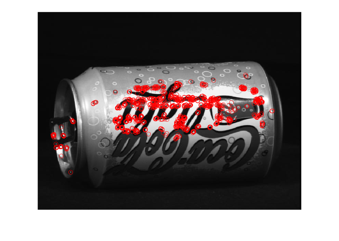
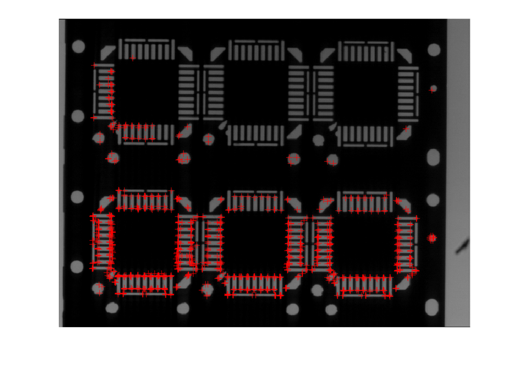
ORB combines fast detection ideas with binary descriptors. It starts from an efficient detector related to FAST, and adds orientation and a compact description of the point neighborhood. Since the descriptor is binary, points can be compared using Hamming distance, which is computationally simple. ORB is therefore widely used when a good balance between speed and quality is needed.

We use the detectORBFeatures command to obtain all ORB-type interest points together with their descriptors. Then we display them over the original image to see what type of features this algorithm detects.

ORB_features_lata_2 = detectORBFeatures(cocacola_lata_2);

puntos_ORB_lata_2 = ORB_features_lata_2.selectStrongest(1000);

puntos_coordenadas_ORB_lata_2 = puntos_ORB_lata_2.Location;

imshow(cocacola_lata_2)
hold on
plot(puntos_coordenadas_ORB_lata_2(:,1),puntos_coordenadas_ORB_lata_2(:,2),'o',Color='r');
hold off

Analysis of the input parameters: scale factor for improving the FAST part of the algorithm, number of octaves, and a region of interest in case the features should be detected in a subregion of the original image.

Another example

ORB_features_frame_1 = detectORBFeatures(frame1);

puntos_ORB_frame_1 = ORB_features_frame_1.selectStrongest(1000);

puntos_coordenadas_ORB_frame_1 = puntos_ORB_frame_1.Location;

imshow(frame1)
hold on
plot(puntos_coordenadas_ORB_frame_1(:,1),puntos_coordenadas_ORB_frame_1(:,2),'+',Color='r')
hold off

Extract features of a certain type and compare them

When descriptors are extracted from two images, matching searches for points with the most similar descriptors. This step gives candidate correspondences, but not all of them must be correct. Different points may have a similar local appearance, especially in repeated textures or poorly distinctive regions. This is why a later geometric verification step is usually added.

The extractFeatures command allows the descriptor vector of the features introduced as an argument to be extracted.

A descriptor is a vector that summarizes the local appearance around an interest point. The detector says where relevant points are; the descriptor says what the neighborhood of those points looks like. This distinction matters because detecting and describing are not exactly the same task.

[descriptor_lata_2, SIFT_features_lata_2] = extractFeatures(cocacola_lata_2,SIFT_features_lata_2);

To compare objects with each other, we repeat the process with the other image containing a can.

SIFT_features_lata_1 = detectSIFTFeatures(cocacola_lata_1);

[descriptor_lata_1, SIFT_features_lata_1] = extractFeatures(cocacola_lata_1,SIFT_features_lata_1);

We compare the two descriptor vectors with the matchFeatures command. If it is binary, the Hamming distance is used, and if not, the normalized Euclidean distance is used. The function returns the indices of the matched features for the two images, and the length command applied to that vector tells us how many features have been matched.

Matching searches, for each descriptor, the most similar descriptor in the other image. For binary descriptors, Hamming distance counts how many bits are different; for real-valued descriptors, numerical distances such as Euclidean distance are used. Good matching should produce many correct correspondences, but it can still include errors.

[indices_pares_features,metrica] = matchFeatures(descriptor_lata_2,descriptor_lata_1,"MatchThreshold",10);

length(indices_pares_features)

ans = 71

We keep only the matched features

matched_SIFT_features_lata_2 = SIFT_features_lata_2(indices_pares_features(:,1),:);
matched_SIFT_features_lata_1 = SIFT_features_lata_1(indices_pares_features(:,2),:);

We display the matching between those features

Displaying the matches is an important qualitative check. If many lines connect coherent parts of the object, the descriptors are working well. If many lines cross without meaning or connect different regions, the geometric verification step is expected to remove those errors.

figure
showMatchedFeatures(cocacola_lata_2,cocacola_lata_1, matched_SIFT_features_lata_2,matched_SIFT_features_lata_1,"montage");

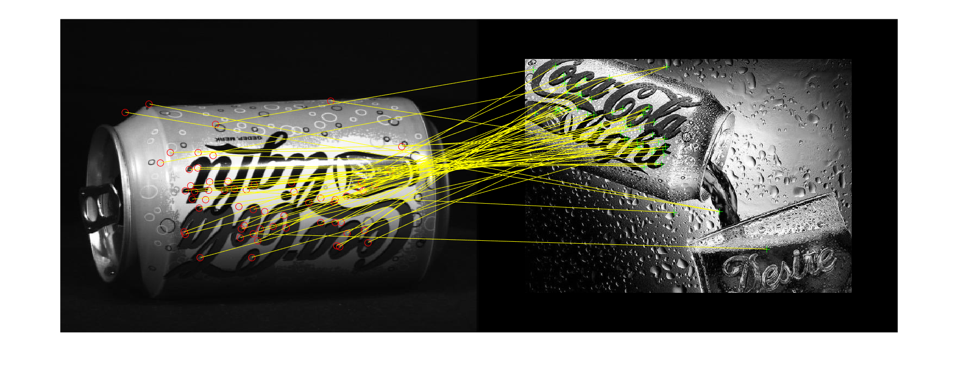
We calculate the geometric transformation (via RANSAC) that allows the geometric alignment between the two images based on the matched features. We use that transformation to transform one of the images and compare the result.

RANSAC is a robust method for estimating a geometric transformation when some correspondences are wrong. It tests different subsets of points and checks which correspondences are consistent with the same transformation model. Consistent correspondences are called inliers, and inconsistent ones are called outliers. In this way, the final alignment depends mainly on reliable matches.

T = estimateGeometricTransform(matched_SIFT_features_lata_2,matched_SIFT_features_lata_1,"affine");

T.T

ans = 3x3 single matrix
   -0.6308   -0.2532         0
    0.2542   -0.6325         0
  329.8466  431.7157    1.0000

cocacola_lata_2_T = imwarp(cocacola_lata_2,T);

montage({cocacola_lata_2_T,cocacola_lata_1})