Tutorial and exercises

WDescriptors are numerical measurements that summarize properties of an object or image region. Instead of comparing all pixels directly, values such as area, perimeter, number of holes or general shape are computed. This makes it easier to compare objects, classify them or use them as input to machine-learning systems.

A descriptor is useful if it preserves the information that matters for the task and ignores variations that should not change the decision. For example, when recognizing a shape, it may be desirable for the descriptor to change little when the object moves, rotates or changes size slightly. This property is called robustness or invariance, depending on the case.

We load the images that we will use in this practical session

monedas = imread("Imagenes\monedas_color.jpg");

monedas = imresize(monedas,[400,400]);

monedas = rgb2gray(monedas);

montage(monedas)

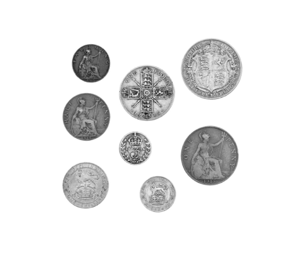
We segment the image. We want a black background, so we take the negative image.

monedas = 255-monedas;

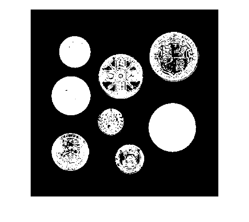
And we binarize using the OTSU method

At this point, Otsu is used to automatically obtain an initial object mask. This mask is not only a final result: it is the basis on which descriptors will be computed. Therefore, if binarization is poor, the descriptors may also be unreliable.

T_otsu = graythresh(monedas);

monedas_bin = imbinarize(monedas,T_otsu);

montage(monedas_bin)

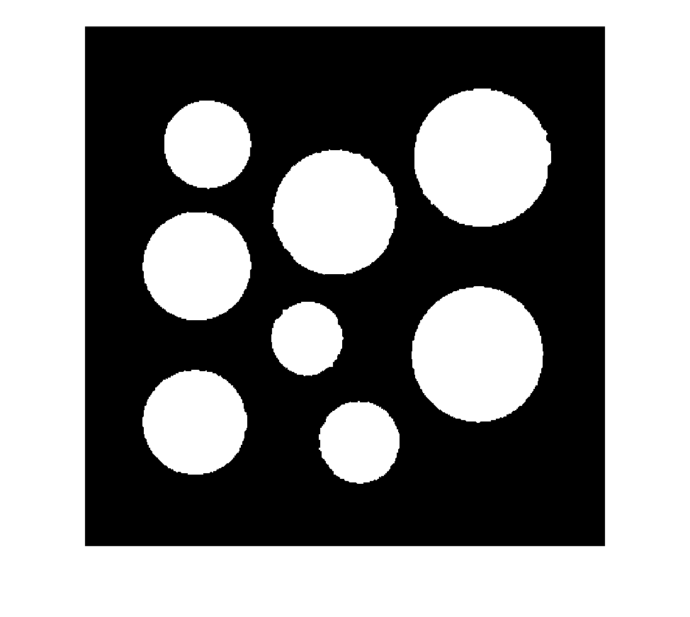
We improve the segmentation using morphological methods for binary images

Descriptor quality strongly depends on the previous segmentation. If the binary mask contains noise, unwanted holes or missing object parts, the computed measurements may be incorrect. This is why morphological operations are often applied before computing descriptors: the goal is to obtain a cleaner and more coherent representation of the object.

monedas_bin = imfill(monedas_bin,"holes");

SE = strel("disk",5);

monedas_bin = imclose(monedas_bin,SE);

montage(monedas_bin)

Topological descriptors

Topological descriptors describe properties related to connectivity. They do not measure exact size or shape; instead, they describe how many components exist, how many holes appear, or how the object structure is organized. This type of descriptor is fairly stable under smooth deformations, as long as the connection between object parts does not change.

Number of connected components.

Counting connected components means counting how many separate objects are present in the binary mask. The result depends on the chosen connectivity and on segmentation quality. Small noise may appear as extra components if it has not been removed beforehand.

numero_componentes_conexas = bwconncomp(monedas_bin).NumObjects

numero_componentes_conexas = 8

comp_conexas = bwlabel(monedas_bin);

Another way to count connected components

numero_componentes_conexas_2 = max(comp_conexas(:))

numero_componentes_conexas_2 = 8

montage({label2rgb(comp_conexas,"jet","k","shuffle")})

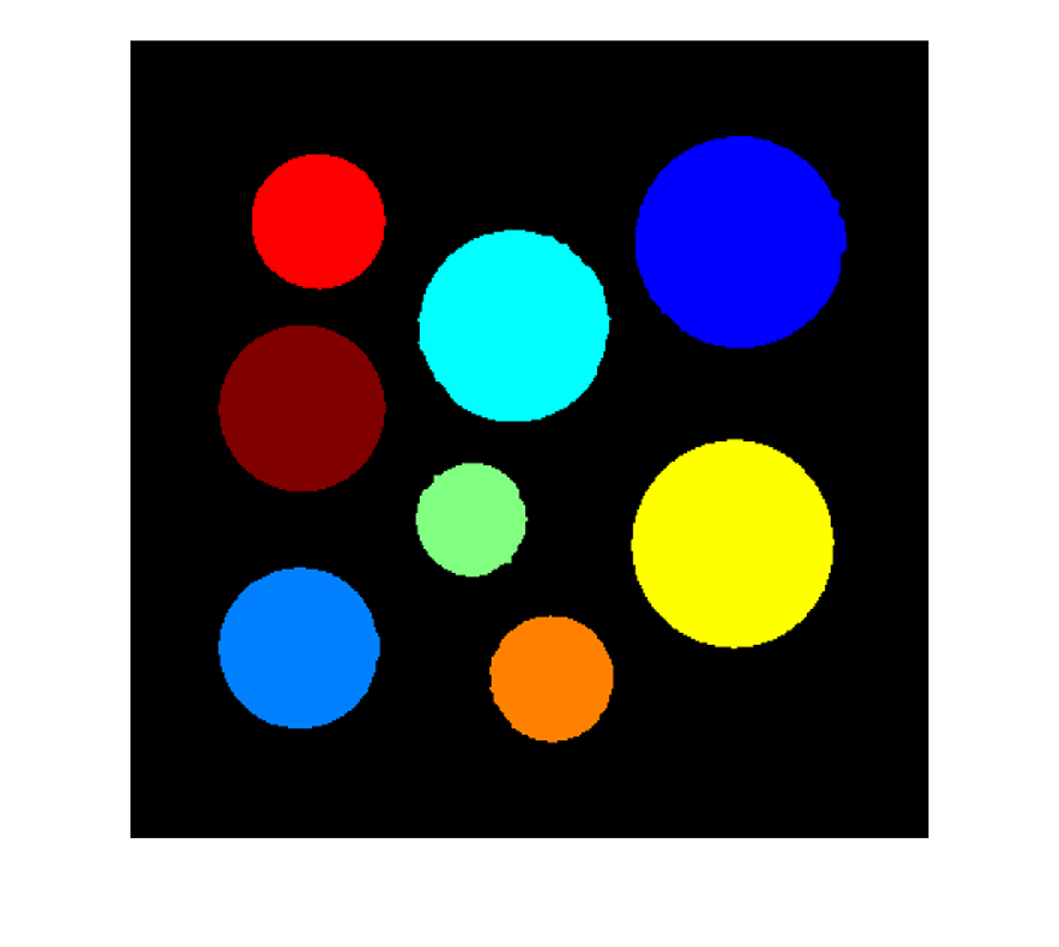
Number of holes. Matlab extracts the borders of each connected component; if there are two borders, it is because one of the borders is internal and surrounds a hole.

The number of holes is a topological descriptor because it describes the internal structure of the object. It does not directly depend on size, but on whether there are background regions completely surrounded by the object. It can be very useful for distinguishing shapes with similar appearance but different topology.

We define an empty vector that will keep count of the holes of each connected component.

agujeros = [];

We iterate through each labeled object or connected component to see if it has holes

for i = 1:numero_componentes_conexas

    comp_i = (comp_conexas == i);

    borde = bwboundaries(comp_i);

    if length(borde) > 1

        agujeros = [agujeros,length(borde)-1];

    end
end

agujeros

agujeros =

     []

Euler characteristic. Remember that the Euler characteristic is the number of connected components that are not black (background) minus the number of holes.

The Euler characteristic combines the number of connected components and the number of holes into a single value. It is a simple measure, but it can be very informative when objects have different topologies. For example, it can help distinguish objects without holes from objects with one or more cavities. However, it does not describe the exact size or shape of the object.

We define an empty vector that will keep count of the Euler characteristic of each connected component.

caracteristica_euler = [];

We iterate through each labeled object or connected component to see what its Euler characteristic is

for i = 1:numero_componentes_conexas

    comp_i = (comp_conexas == i);

    borde = bwboundaries(comp_i);

    caracteristica_euler = [caracteristica_euler,1-(length(borde)-1)];

end

caracteristica_euler

caracteristica_euler = 1x8
     1     1     1     1     1     1     1     1

Another example

figuras_agujeros = imread("Imagenes\figuras_agujeros.png");

figuras_agujeros = rgb2gray(figuras_agujeros);

T_otsu_figuras = graythresh(figuras_agujeros);

figuras_agujeros_bin = imbinarize(figuras_agujeros,T_otsu_figuras);

montage(figuras_agujeros_bin)

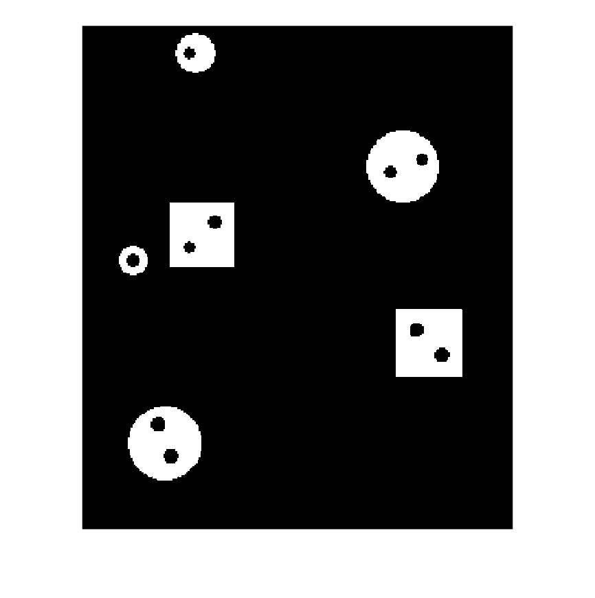
numero_comps_conexas = bwconncomp(figuras_agujeros_bin).NumObjects

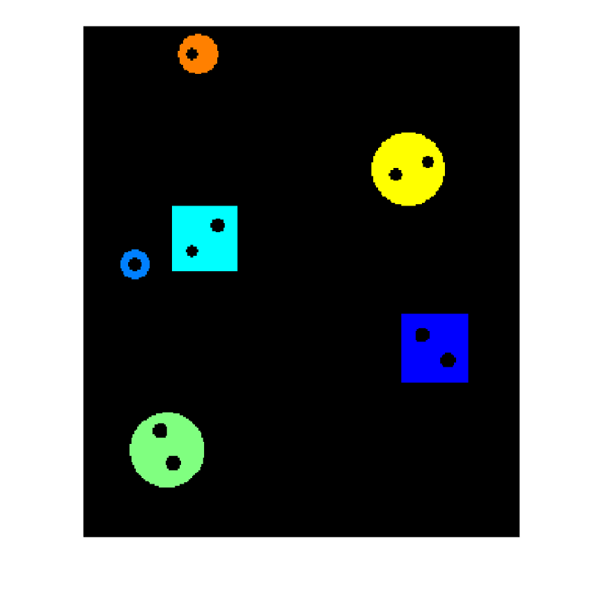
numero_comps_conexas = 6

comp_conexas_figuras = bwlabel(figuras_agujeros_bin);

montage({label2rgb(comp_conexas_figuras,"jet","k","shuffle")})

agujeros_2 = [];
caracteristica_euler_2 = [];

for i = 1:numero_comps_conexas

    comp_i = (comp_conexas_figuras == i);

    borde = bwboundaries(comp_i);

    if length(borde) > 1

        agujeros_2 = [agujeros_2,length(borde)-1];
        caracteristica_euler_2 = [caracteristica_euler_2,1-(length(borde)-1)];

    end
end

agujeros_2

agujeros_2 = 1x6
     1     2     2     1     2     2

caracteristica_euler_2

caracteristica_euler_2 = 1x6
     0    -1    -1     0    -1    -1

Skeleton calculation. Calculation based on the distance transform

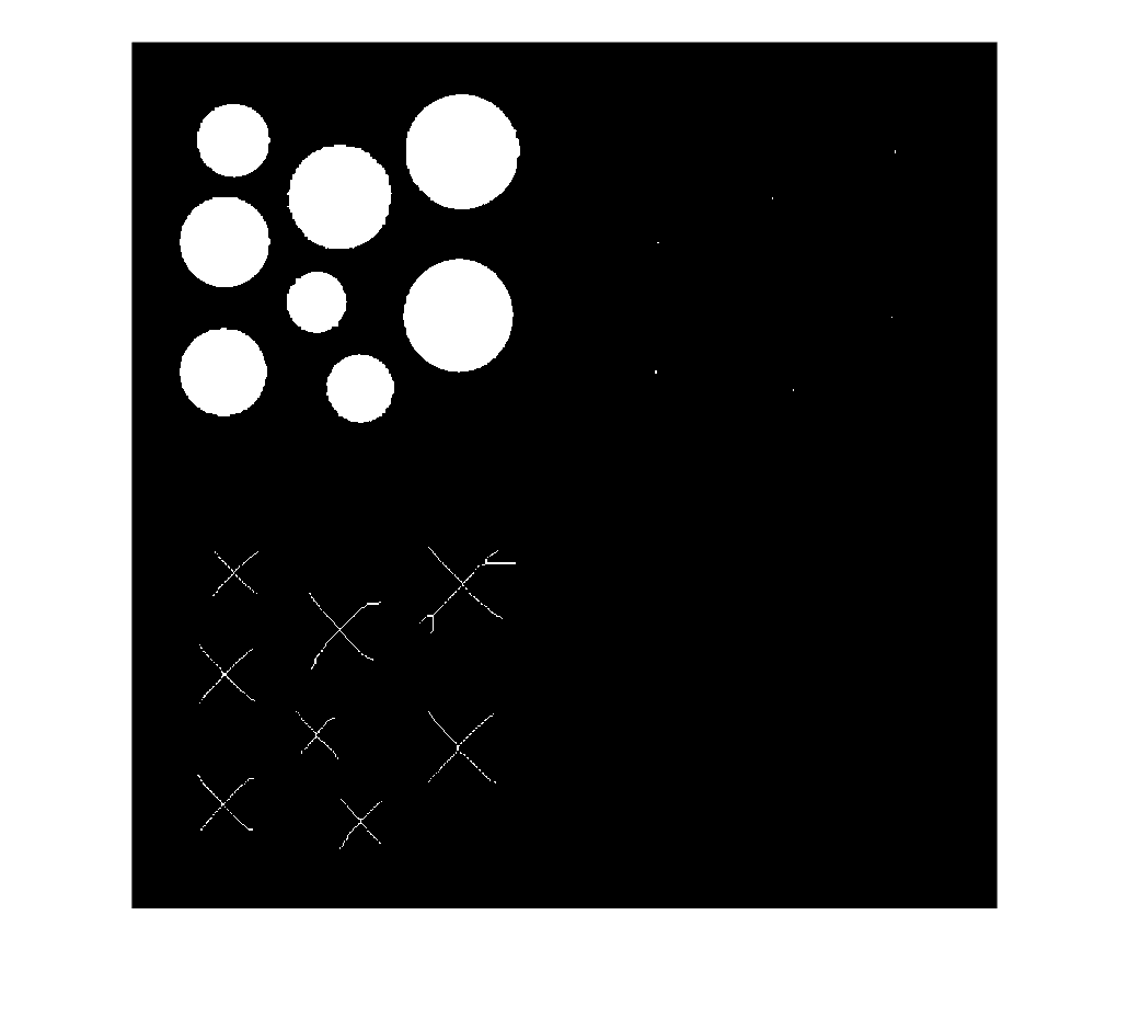
The skeleton is a simplified representation of an object shape. The idea is to reduce the object to a central, thin and connected structure that preserves its general organization. This representation can be useful for studying elongated or branched objects. However, small contour irregularities can create additional branches that do not always have real meaning.

monedas_skel = bwskel(monedas_bin);

Calculation based on thinning with morphological operators

monedas_skel_2 = bwmorph(monedas_bin,"skeleton",Inf);

montage({monedas_bin,monedas_skel,monedas_skel_2})

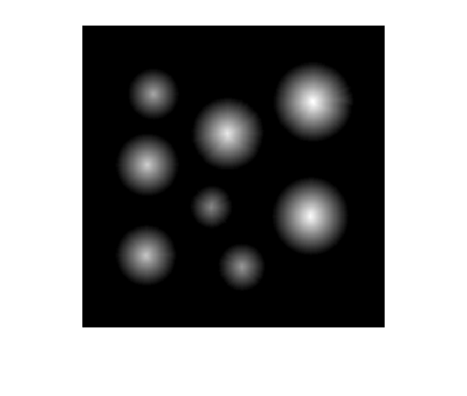
Calculation of the distance transform

D = bwdist(~monedas_bin);

imshow(D,[])

Geometric descriptors

Geometric descriptors measure properties related to object size, position and shape. Some, such as area and perimeter, depend directly on the image scale. Others, such as compactness or eccentricity, describe proportions and may be more useful for comparing objects of different sizes.

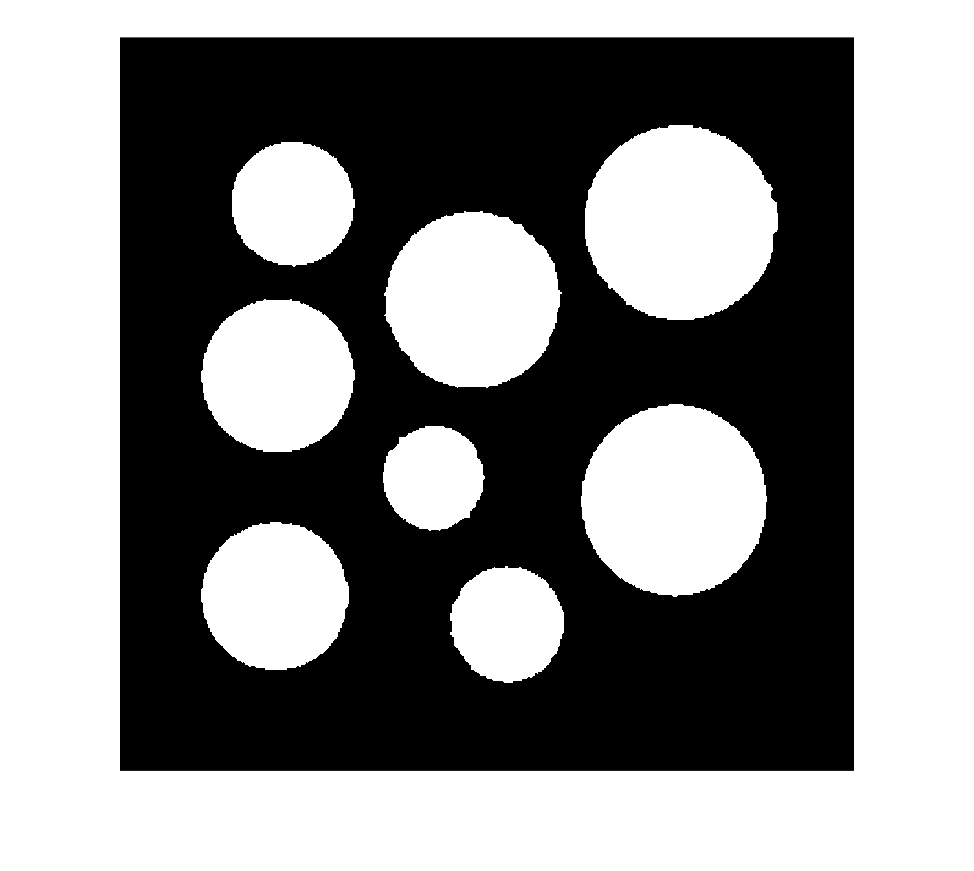
montage(monedas_bin)

Area calculation.

Area is computed by counting the pixels that belong to the object. It is a simple size measurement, but it depends on image scale and resolution. If two images have different scales, area must be normalized or interpreted carefully.

We define an empty vector that will calculate the area of each connected component.

area = [];

We iterate through each labeled object or connected component to see what its area is

for i = 1:numero_componentes_conexas

    comp_i = (comp_conexas == i);

    area = [area,sum(comp_i(:))];

end

area

area = 1x8
        5453        5074        3563        2436        7174        3047        8253        8731

Perimeter calculation.

Perimeter measures the length of the object contour. Unlike area, it is very sensitive to boundary irregularities: a noisy contour may have an artificially large perimeter. This is why it is often useful to clean the mask before computing it.

perimetro = [];

for i = 1:numero_componentes_conexas

    comp_i = (comp_conexas == i);

    perimetro = [perimetro,regionprops(comp_i, 'Perimeter').Perimeter];

end

perimetro

perimetro = 1x8
  258.9320  250.6950  209.2860  175.7500  301.8050  196.0870  320.1980  332.9510

Like the perimeter, the area can also be calculated with the command regionprops(comp_i, 'Area').Area]

Centroid or center of mass calculation

The centroid is the average position of the object if all its pixels had the same weight. It summarizes object location with a single point. It is useful for tracking, shape comparison and computing spatial relationships between objects.

centroide = [];

for i = 1:numero_componentes_conexas

    comp_i = (comp_conexas == i);

    centroide = [centroide;regionprops(comp_i, 'Centroid').Centroid];

end

centroide

centroide = 8x2
   86.5034  185.0011
   85.0530  305.2221
   94.6444   91.2088
  171.4179  240.7373
  192.8400  143.6901
  211.6853  320.4207
  302.5620  252.9773
  305.9201  101.5368

Compactness calculation

Compactness relates the area of an object to its perimeter. A rounded object with a smooth contour is usually more compact than a very elongated object or one with many irregularities. Therefore, this measurement can provide information about shape complexity, even though it does not describe every contour detail.

compacidad = perimetro.*perimetro./area

compacidad = 1x8
   12.2952   12.3863   12.2932   12.6798   12.6967   12.6190   12.4230   12.6969

Diameter calculation

diametro = [];

for i = 1:numero_componentes_conexas

    comp_i = (comp_conexas == i);

    diametro = [diametro,regionprops(comp_i, 'MajorAxisLength').MajorAxisLength];

end

diametro

diametro = 1x8
   83.5045   80.6870   67.6135   56.6321   96.2877   63.1585  104.0661  106.1058

Eccentricity calculation (that is, the major axis-minor axis ratio)

Eccentricity describes how elongated a shape is. An object close to a circle has low eccentricity, while an elongated object has high eccentricity. This measure is useful because it describes shape proportion and not only absolute size.

diametro_menor = [];

for i = 1:numero_componentes_conexas

    comp_i = (comp_conexas == i);

    diametro_menor = [diametro_menor,regionprops(comp_i, 'MinorAxisLength').MinorAxisLength];

end

excentricidad = diametro./diametro_menor

excentricidad = 1x8
1.0041    1.0074    1.0074    1.0328    1.0146    1.0274    1.0304    1.0124

Bounding box calculation

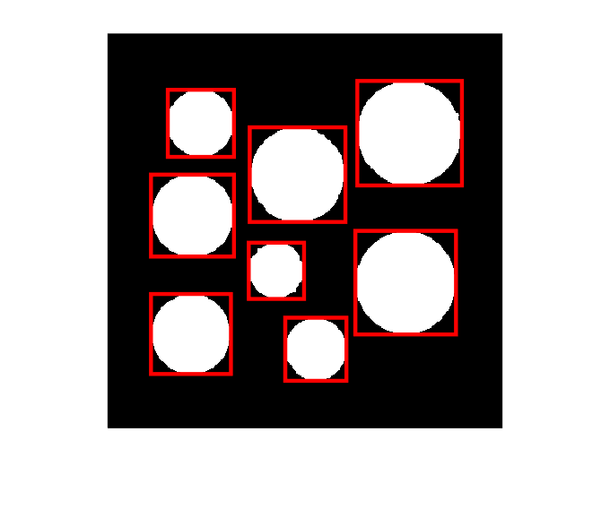
The bounding box is the simplest rectangle that approximately locates an object in the image. It does not describe the exact contour, but it summarizes position, width and height in a practical way. This idea is also fundamental in deep-learning object detection, where predicted boxes are compared with annotations using measures such as IoU.

imshow(monedas_bin);
hold on;

for i = 1:numero_componentes_conexas

    comp_i = (comp_conexas == i);

    bounding_box = regionprops(comp_i, 'boundingbox').BoundingBox;

    rectangulo = rectangle('Position', bounding_box, 'EdgeColor', 'r', 'LineWidth', 2);

end

hold off