Tutorial and exercises

Introduction

From an image-processing point of view, a filter modifies an image by computing new values for its pixels. In many cases, the new value depends on the surrounding pixels, that is, on a local neighborhood. When this combination is linear, it can be described as a convolution with a small matrix of weights called a kernel.

Although this practical mainly works in the spatial domain, the frequency interpretation is also useful. Slow variations correspond to smooth image regions, while fast variations usually appear at edges, textures or noise. Smoothing filters reduce these fast variations, whereas enhancement filters make them more visible.

In this practical assignment, different smoothing and enhancement filters applied to grayscale images are studied. The objective is to understand how these filters act, both mathematically and visually, and to analyze their behavior in the presence of noise.

Basic image manipulation

We load the images that will be used throughout the practical assignment and convert them to grayscale when necessary, in order to work only with intensity levels.

lena = imread("Imagenes\lena_gray_512.tif");

universo = imread("Imagenes\Universo.jpg");

universo = rgb2gray(universo);

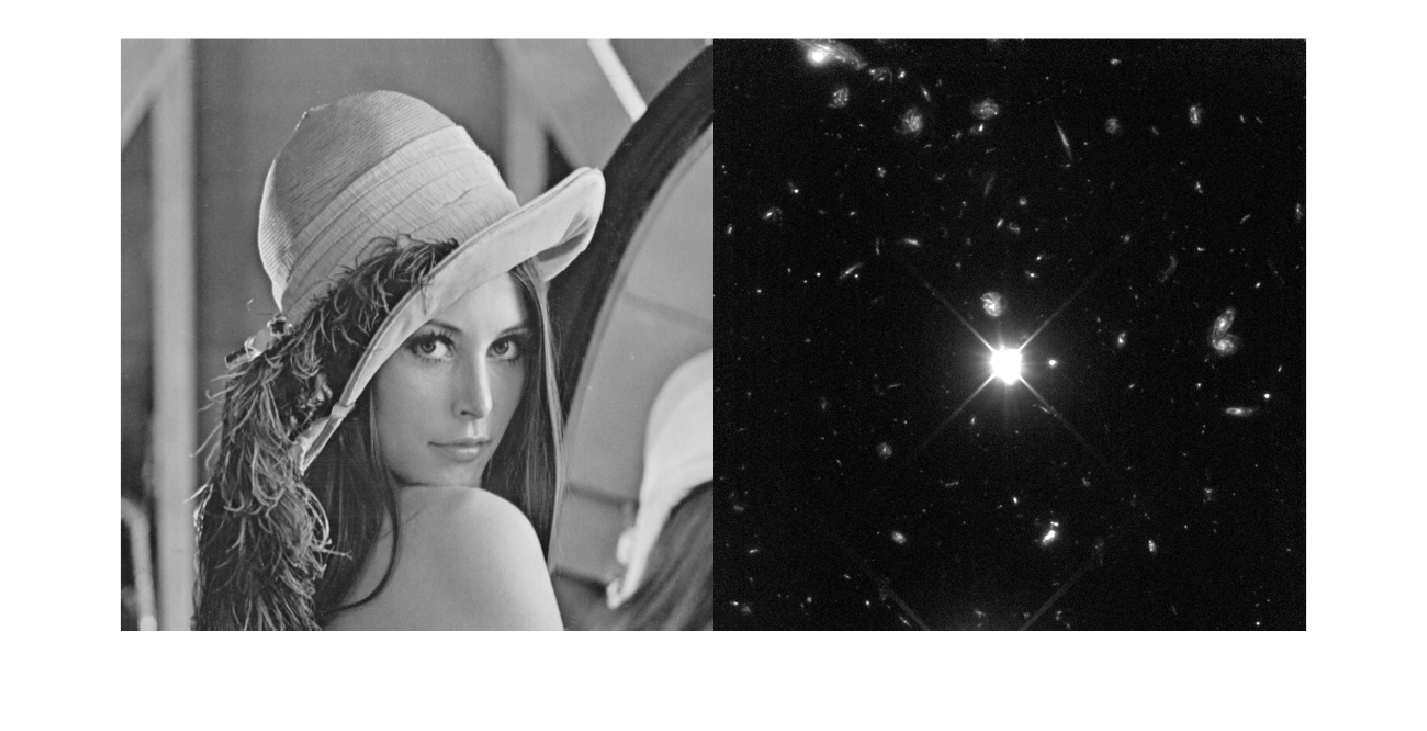
We display the loaded images to check that they have been read correctly.

montage({lena,universo})

Smoothing filters

Smoothing filters reduce noise and abrupt intensity variations, at the cost of losing fine detail in the image.

The neighborhood size and the kernel weights determine how strongly the image is modified. A small neighborhood preserves detail better, but may remove little noise. A large neighborhood smooths more, but may also remove weak edges or small structures that could be important in a later segmentation step.

Convolution product. We define a 3x3 mean kernel, which assigns the same weight to all pixels in the neighborhood.

The mean filter replaces each pixel with the average value of its neighborhood. This reduces small variations and random noise, but it can also blur edges because it mixes pixels from different sides of a contour.

w = (1./9.)*[1,1,1;1,1,1;1,1,1];

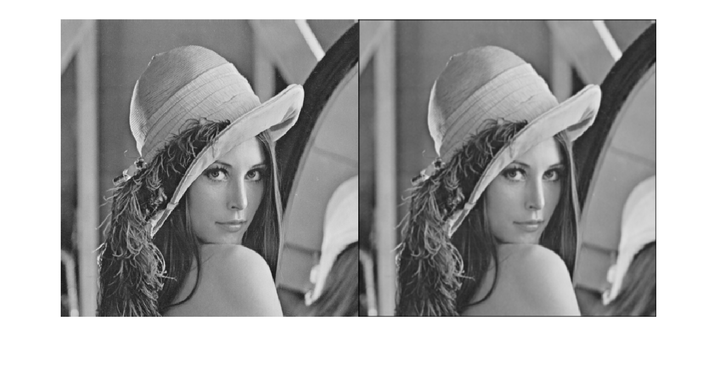
We apply the convolution using conv2. This function does not automatically handle borders, which causes visible artifacts.

lena_conv = conv2(lena,w);

montage({lena,uint8(lena_conv)}) % Observe the borders

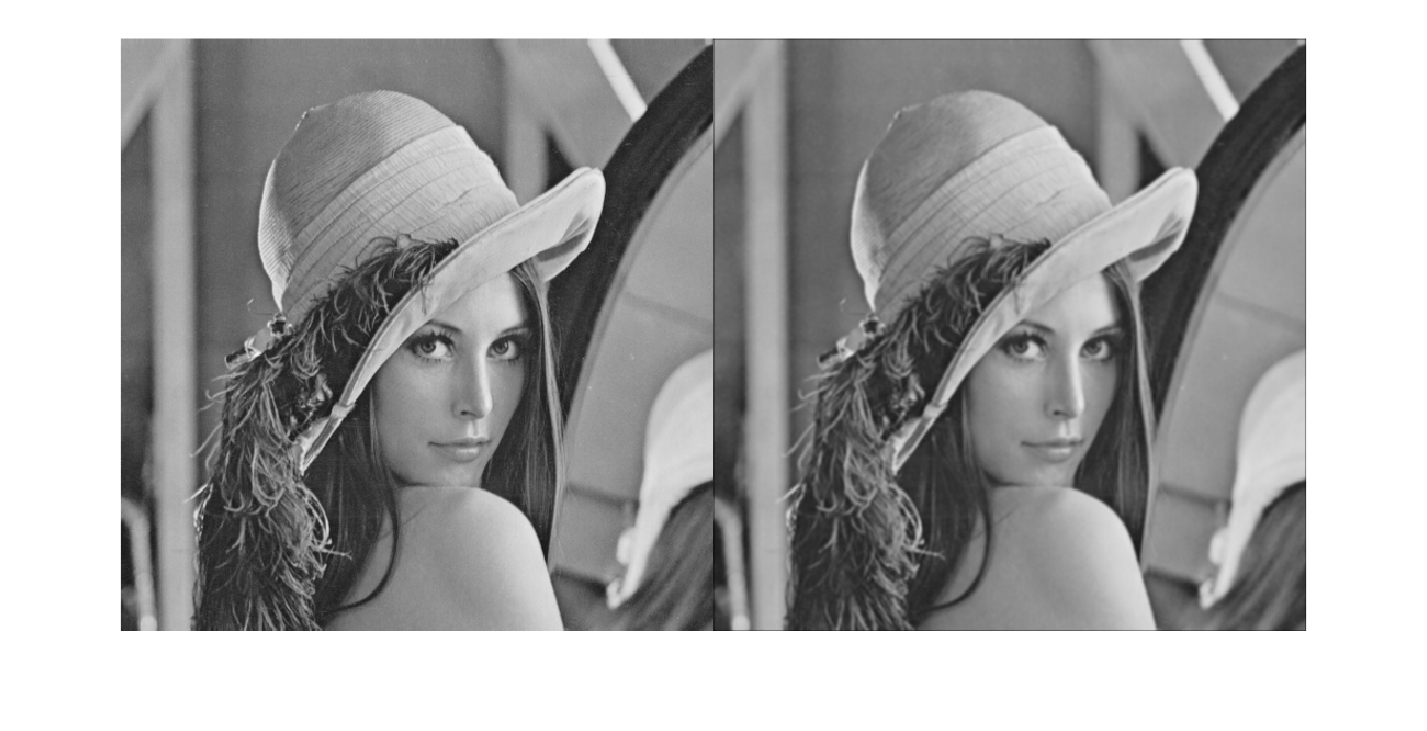
Mean filter using imfilter. The imfilter function allows the same kernel to be applied, but with better border handling.

lena_media = imfilter(lena,w);

montage({lena,lena_media})

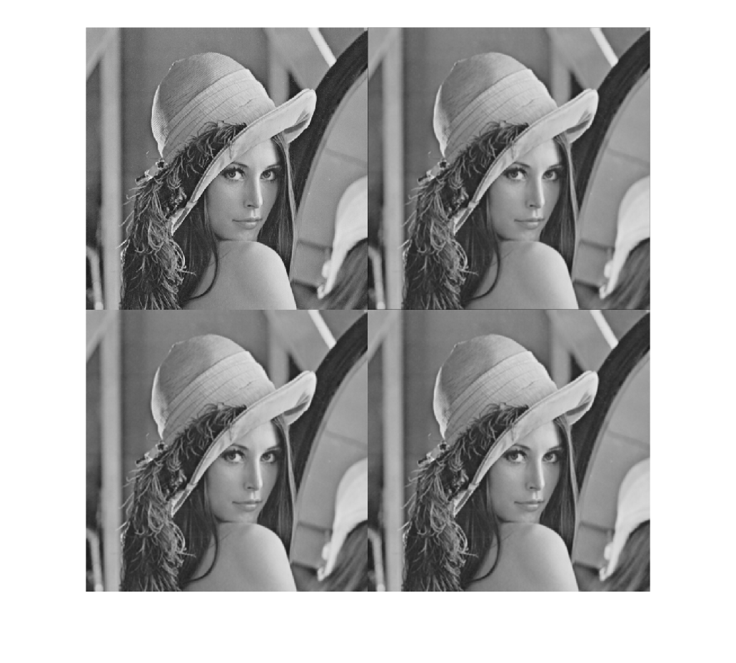
Padding in imfilter. By default, zero-padding is used, but other options can be used to improve the result at the borders.

lena_media_r = imfilter(lena,w,'replicate');

lena_media_s = imfilter(lena,w,'symmetric');

montage({lena,lena_media,lena_media_r,lena_media_s}) % Compare especially the borders

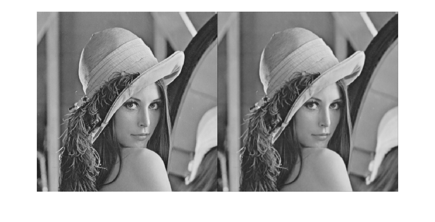
Gaussian filter. The Gaussian filter assigns more weight to the central pixel and smooths in a more natural way.

A Gaussian filter is a smoothing filter based on the Gaussian distribution. Pixels close to the center of the kernel have more weight than distant pixels, so the smoothing is more gradual than with a uniform average. The sigma parameter controls the width of the Gaussian: the larger sigma is, the stronger the smoothing becomes and the more fine details may be lost.

3x3 Gaussian kernel with sigma = 1

w_gaussian = (1./16.)*[1,2,1;2,4,2;1,2,1];

lena_gaussian = imfilter(lena,w_gaussian);

montage({lena,lena_gaussian})

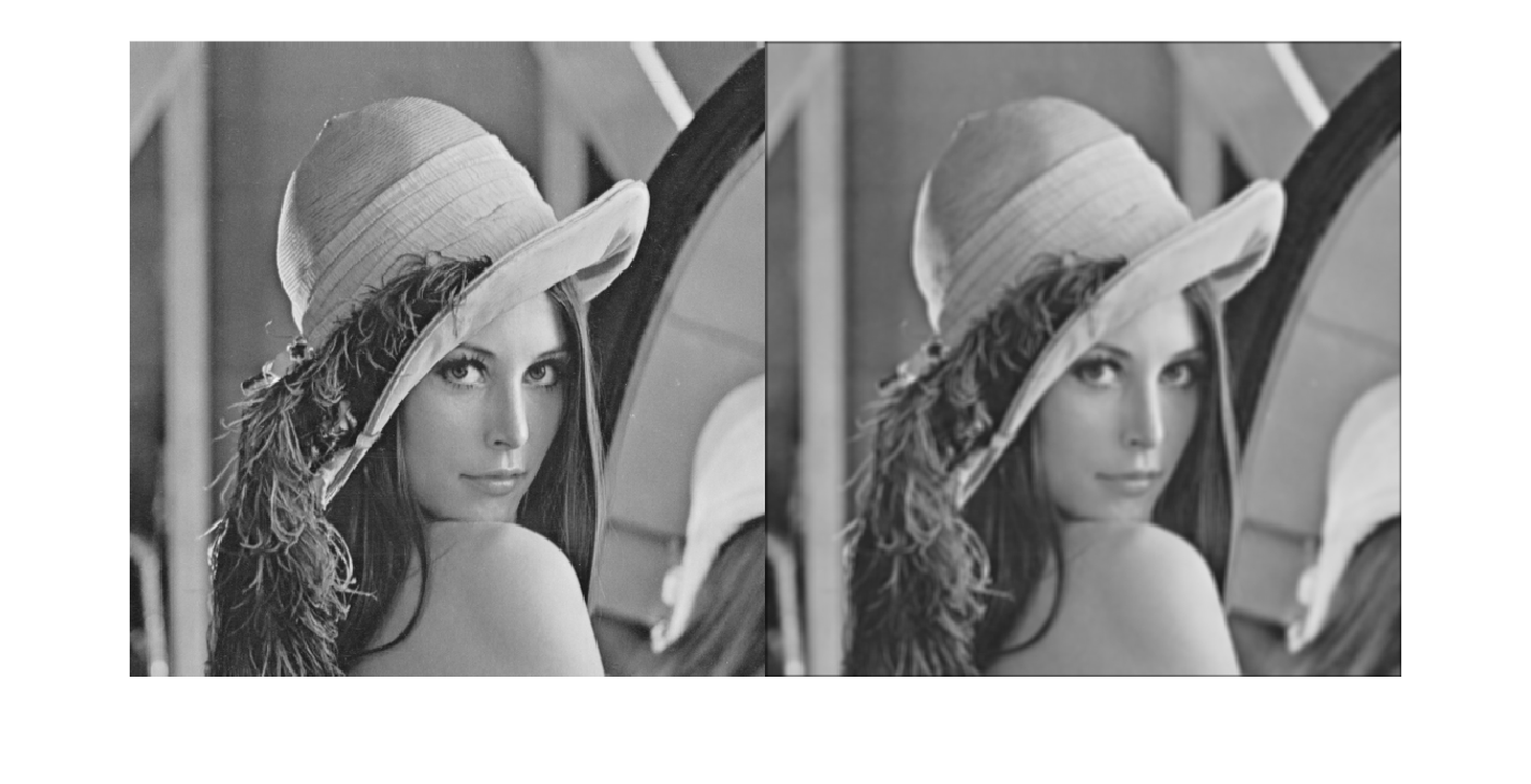
Larger Gaussian filters using fspecial

When a larger Gaussian kernel is used, the filter can take a wider neighborhood into account. This is useful when noise is important, but it also increases the risk of removing fine textures or weak edges. For this reason, kernel size and sigma should be chosen according to the scale of the details that should be preserved.

w_gaussian = fspecial("gaussian",5,5);

lena_gaussian = imfilter(lena,w_gaussian);

montage({lena,lena_gaussian})

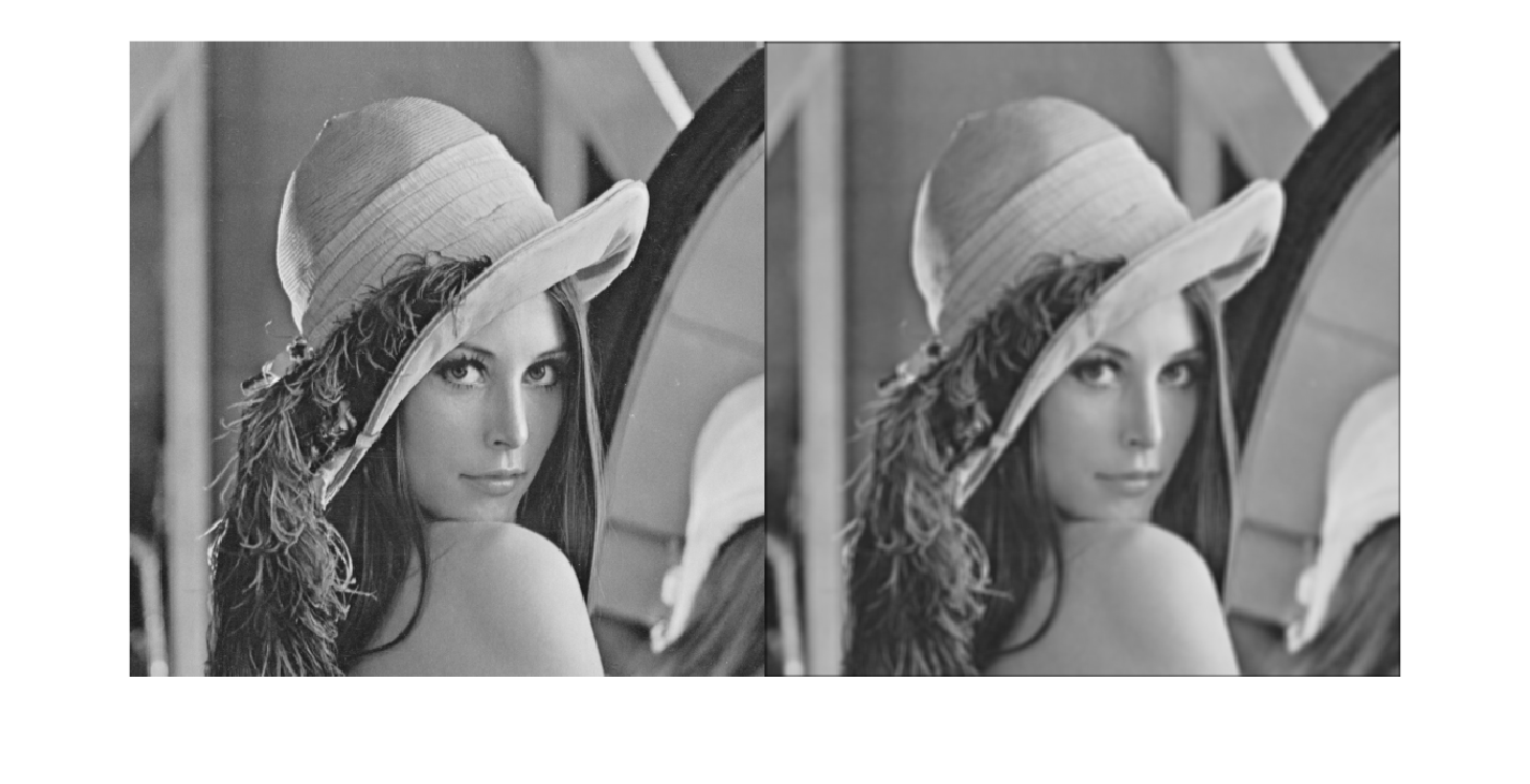
Generic mean filter with fspecial

w_media = fspecial("average",5);

lena_media = imfilter(lena,w_media);

montage({lena,lena_media})

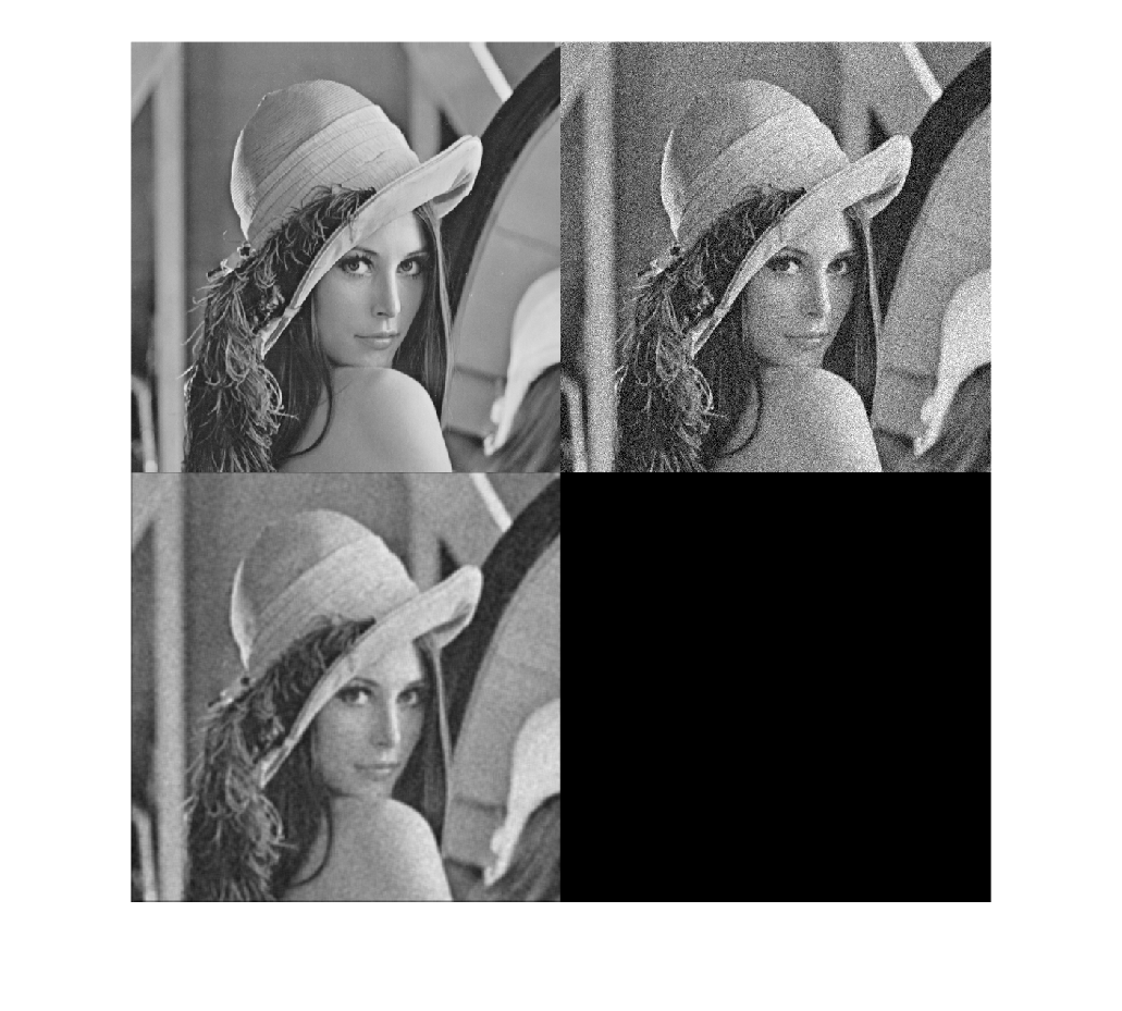
Application of the mean filter for Gaussian noise reduction. First, we add Gaussian noise and then apply the filter to observe its effect.

lena_ruido = imnoise(lena,"gaussian",0,0.01);

lena_ruido_fil = imfilter(lena_ruido,w_media);

montage({lena,lena_ruido,lena_ruido_fil})

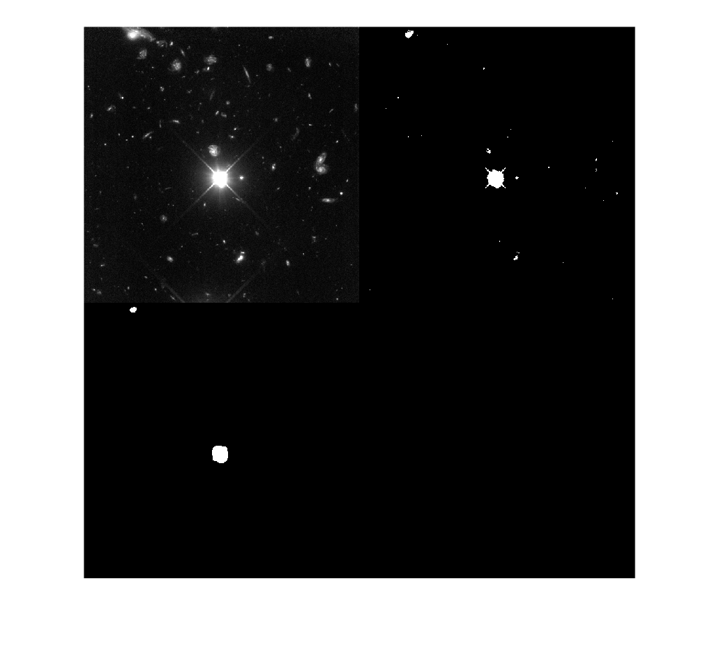
Pre-smoothing to improve binarization. Smoothing reduces small variations and enables more stable binarization.

universo_bin = universo>200;

w_media = fspecial("average",25);

universo_fil = imfilter(universo,w_media);

universo_fil_bin = universo_fil>200;

montage({universo,universo_bin,universo_fil_bin})

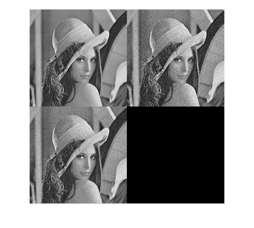
Application of the Gaussian filter to noise reduction

w_gausiano = fspecial("gaussian",3,3);

lena_ruido_fil = imfilter(lena_ruido,w_gausiano);

montage({lena,lena_ruido,lena_ruido_fil})

Statistical filters

Statistical filters also examine a local neighborhood, but they do not compute the result as a weighted sum. Instead, they use a statistic such as the minimum, maximum or median. This difference makes them more suitable when there are outlier values, as happens with salt-and-pepper noise.

These filters are based on local statistics of the neighborhood.

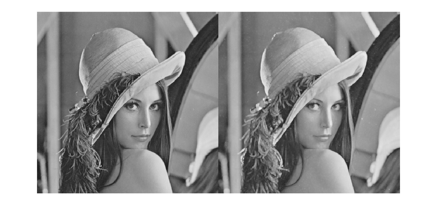
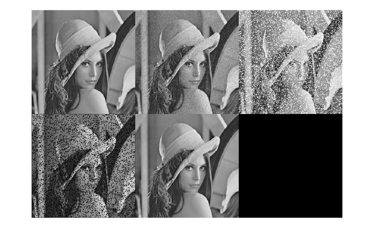
Maximum filter. It enhances bright areas and removes isolated dark points.

The maximum filter assigns each pixel the highest value in its neighborhood. It therefore expands bright regions and can remove small dark points. It is a nonlinear operation and is related to grayscale morphological dilation.

w_estadistico = ones(3);

lena_max = ordfilt2(lena,numel(w_estadistico),w_estadistico);

montage({lena,lena_max})

Minimum filter. It enhances dark areas and removes isolated bright points.

The minimum filter performs the opposite operation: it assigns each pixel the lowest value in its neighborhood. This expands dark regions and can remove small bright points. Conceptually, it is similar to grayscale morphological erosion.

lena_min = ordfilt2(lena,1,w_estadistico);

montage({lena,lena_min})

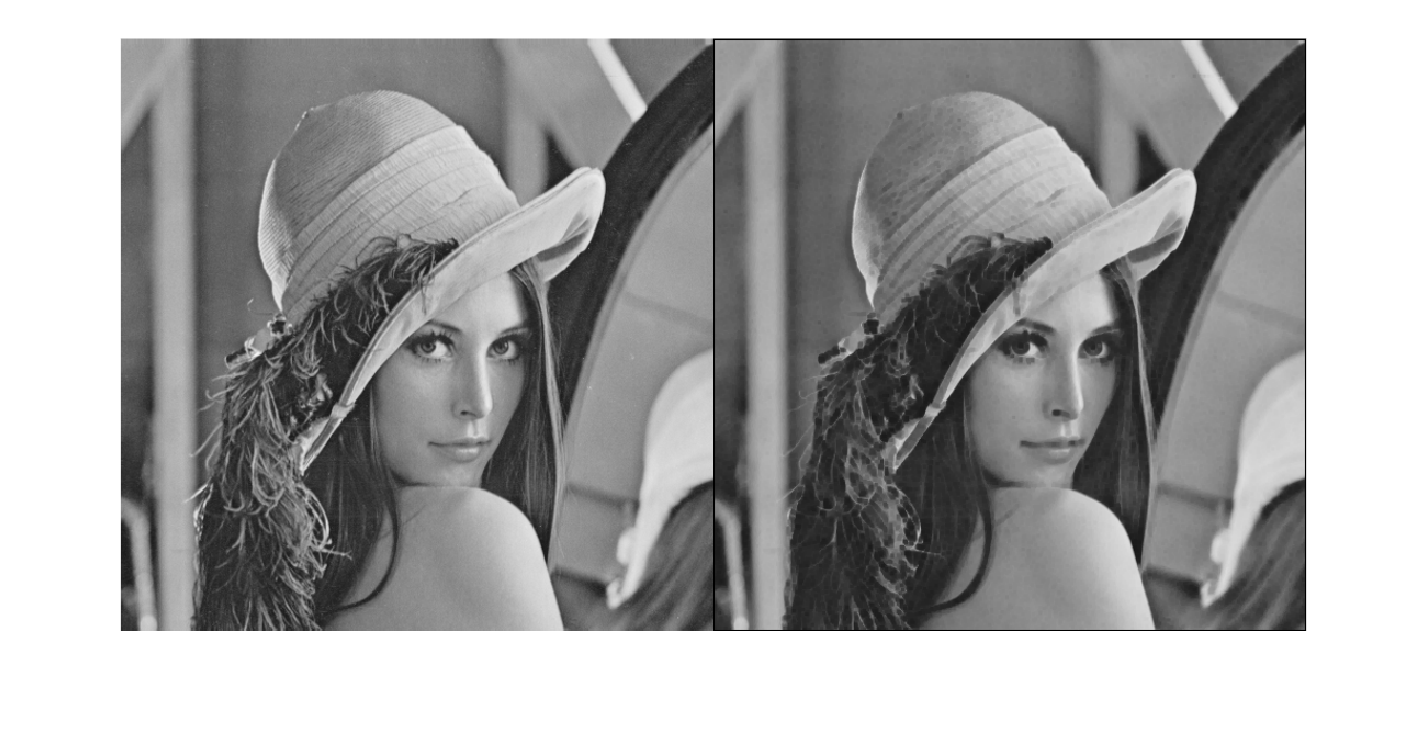
Median filter. It is especially effective for removing impulse noise (salt and pepper).

The median filter sorts the values in the neighborhood and selects the central value. Since it does not compute an average, extreme values produced by salt-and-pepper noise have less influence. This is why it often preserves edges better than the mean filter when the noise is impulsive.

lena_mediana = medfilt2(lena,size(w_estadistico));

montage({lena,lena_mediana})

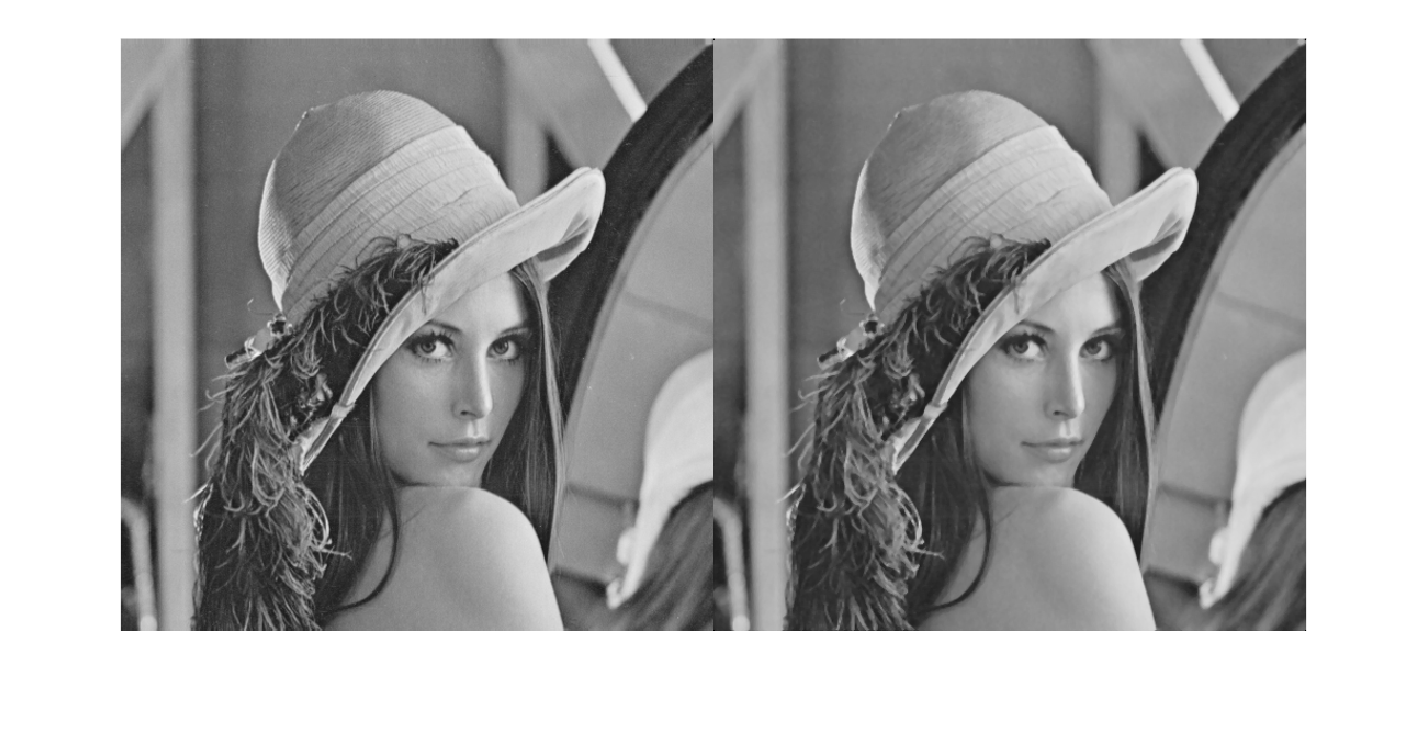
Application of statistical filters to salt and pepper noise

probabilidad = 0.05;

ruido_impulsional = rand(size(lena));

lena_con_ruido = lena;

lena_con_ruido(ruido_impulsional < probabilidad/2) = 0;

lena_con_ruido(ruido_impulsional > 1 - probabilidad/2) = 255;

lena_max = ordfilt2(lena_con_ruido,numel(w_estadistico),w_estadistico);

lena_min = ordfilt2(lena_con_ruido,1,w_estadistico);

lena_mediana = medfilt2(lena_con_ruido,size(w_estadistico));

montage({lena,lena_con_ruido,lena_max,lena_min,lena_mediana})

Enhancement filters

Enhancement filters aim to highlight important intensity changes. These changes may correspond to object boundaries, texture changes, shadows or discontinuities in the scene. Since noise can also produce abrupt changes, it is common to smooth the image before computing gradients or derivatives.

These filters highlight abrupt changes in intensity and allow edges to be detected.

Digital derivative by definition. The derivatives in the x and y directions are approximated using simple kernels.

w_dx = [0,1,0;0,-1,0;0,0,0];
w_dy = [0,0,0;1,-1,0;0,0,0];

Digital gradient. The magnitude of the derivatives in both directions is combined.

The gradient measures how intensity changes in the horizontal and vertical directions. Its magnitude is large where there is a strong transition, such as an edge. This makes the gradient a basic tool for detecting contours and orienting other descriptors.

lena_gradiente = abs(imfilter(lena,w_dx)) + abs(imfilter(lena,w_dy));

lena_negativa = 255 - lena_gradiente;

montage({lena,lena_gradiente,lena_negativa})

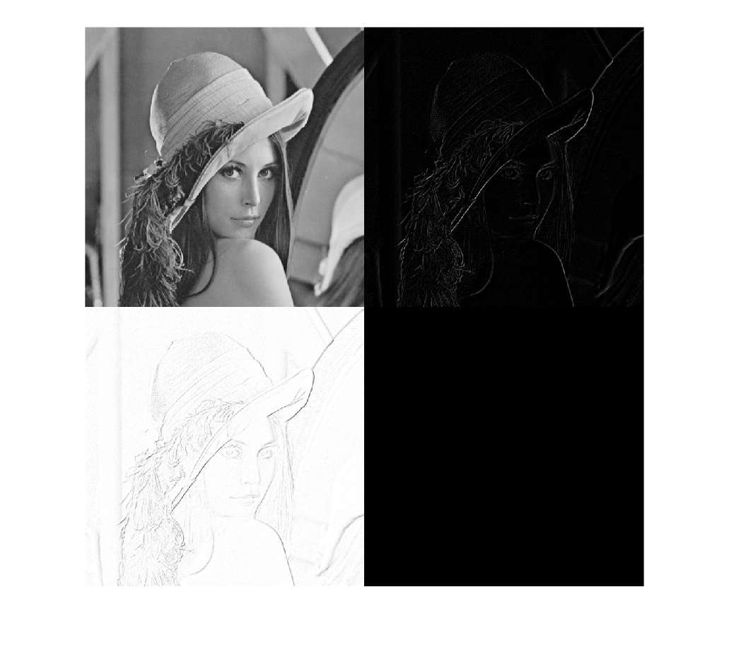
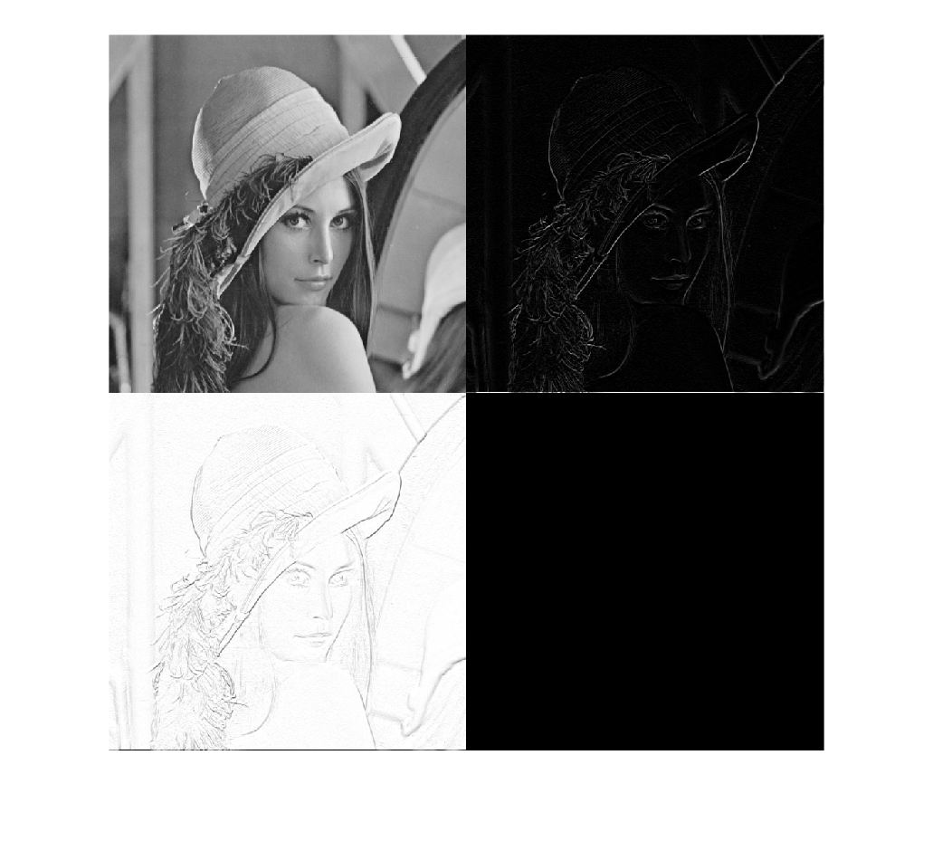
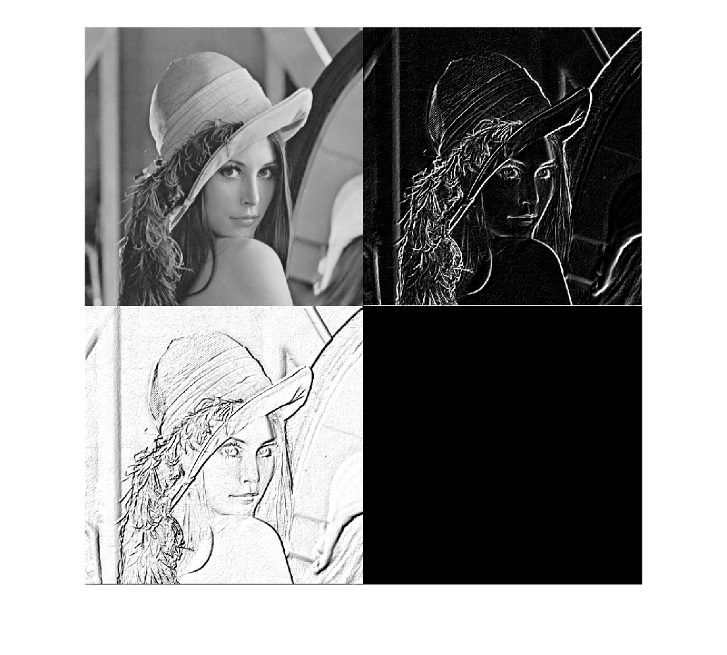
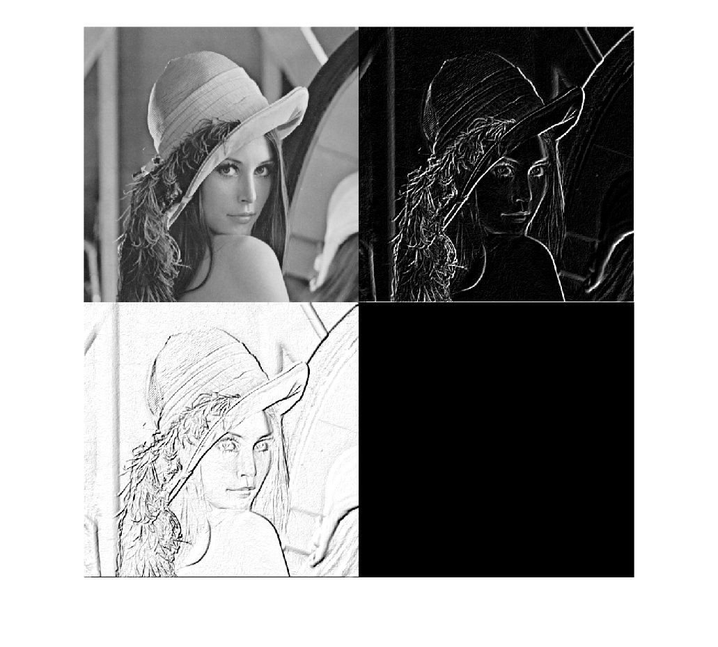
Roberts, Sobel and Prewitt filters. These filters calculate the gradient using different approximations.

Roberts, Sobel and Prewitt are discrete approximations of the image derivative. Roberts is more local and can be more sensitive to noise, while Sobel and Prewitt include some smoothing in the perpendicular direction. This often makes edge detection more stable, although the response may vary depending on edge orientation.

Roberts filter

wR_dx = [1,0;0,-1];
wR_dy = [0,1;-1,0];

lena_gradiente_roberts = abs(imfilter(lena,wR_dx)) + abs(imfilter(lena,wR_dy));

lena_negativa_roberts = 255 - lena_gradiente_roberts;

montage({lena,lena_gradiente_roberts,lena_negativa_roberts})

Sobel filter

w_sobel = fspecial("sobel");

lena_gradiente_sobel = abs(imfilter(lena,w_sobel)) + abs(imfilter(lena,w_sobel'));

lena_negativa_sobel = 255 - lena_gradiente_sobel;

montage({lena,lena_gradiente_sobel,lena_negativa_sobel})

Prewitt filter

w_prewitt = fspecial("prewitt");

lena_gradiente_prewitt = abs(imfilter(lena,w_prewitt)) + abs(imfilter(lena,w_prewitt'));

lena_negativa_prewitt = 255 - lena_gradiente_prewitt;

montage({lena,lena_gradiente_prewitt,lena_negativa_prewitt})

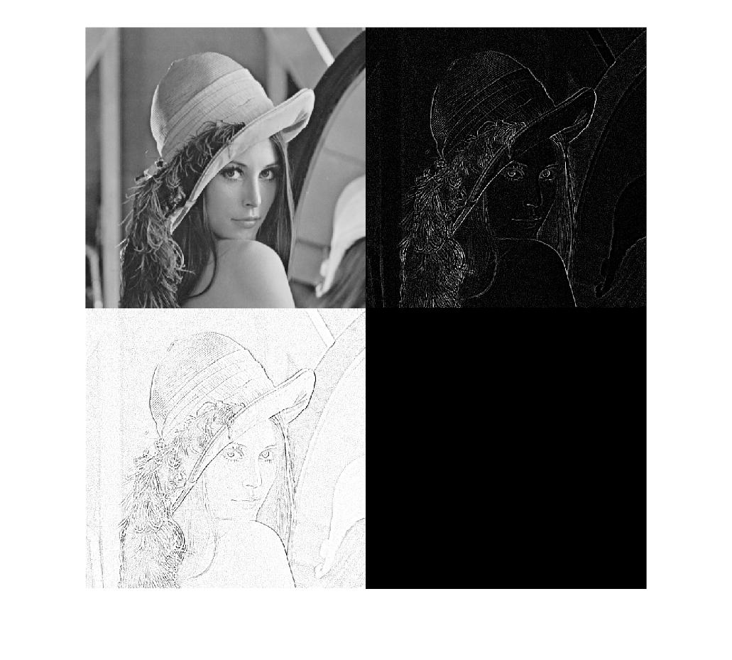
Digital Laplacian. It detects intensity changes in all directions.

The Laplacian is a second-order derivative. Unlike the gradient, it does not provide a main direction of change, but responds to intensity variations in any orientation. Because second-order derivatives are very sensitive to noise, they are often combined with previous smoothing, as in the Laplacian of Gaussian filter.

w_laplaciano = [1,1,1;1,-8,1;1,1,1];

lena_laplaciano = imfilter(lena,w_laplaciano);

lena_laplaciano_negativo = 255 - lena_laplaciano;

montage({lena,lena_laplaciano,lena_laplaciano_negativo})

Laplacian of Gaussian (LoG). It combines Gaussian smoothing and edge detection.

LoG first applies Gaussian smoothing and then a Laplacian. The smoothing reduces the response to noise, while the Laplacian detects fast intensity changes. This combination is useful because second-order derivatives are very sensitive to noise when applied directly.

w_ruido_gauss = fspecial('gaussian',3,1);

lena_ruido_gauss = imfilter(lena,w_ruido_gauss);

lena_log = imfilter(lena_ruido_gauss,w_laplaciano);

lena_log_negativo = 255 - lena_log;

montage({lena,lena_laplaciano,lena_laplaciano_negativo,lena_log,lena_log_negativo})

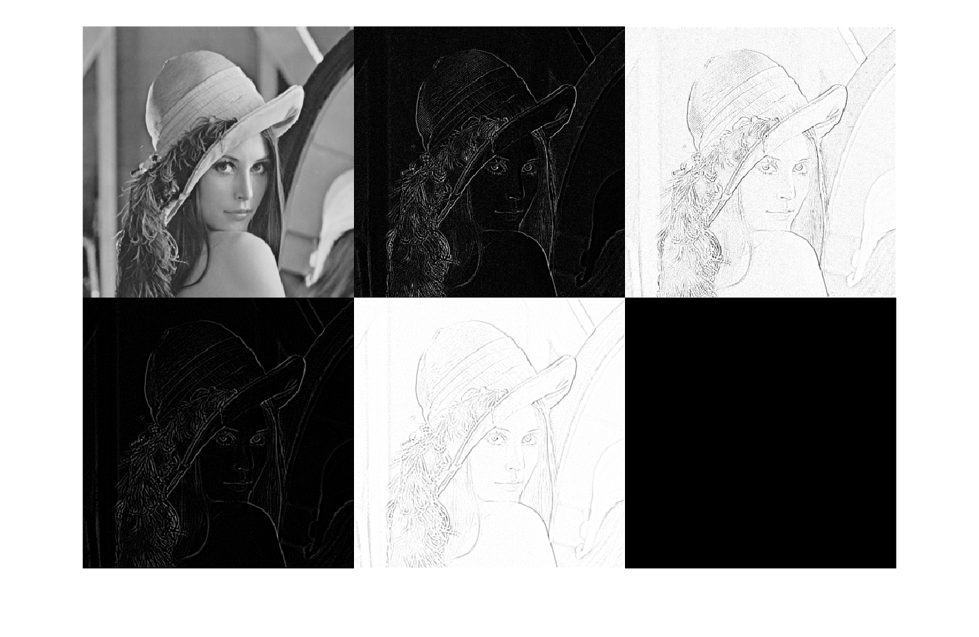
Difference of Gaussians (DoG). The result of two Gaussian filters with different sigma values is subtracted.

Difference of Gaussians compares two smoothed versions of the image obtained with different sigma values. Subtracting them highlights structures visible at a certain scale and reduces other details. This idea of working at different scales is very important in computer vision, especially in interest-point detectors such as SIFT.

sigma1 = 0.5;
sigma2 = 2;

w_gaussiano1 = fspecial('gaussian',9,sigma1);
w_gaussiano2 = fspecial('gaussian',9,sigma2);

lena_gaussiano_1 = imfilter(lena,w_gaussiano1);
lena_gaussiano_2 = imfilter(lena,w_gaussiano2);

lena_dog = lena_gaussiano_2 - lena_gaussiano_1;

lena_dog_negativa = 255 - lena_dog;

montage({lena,lena_dog,lena_dog_negativa})

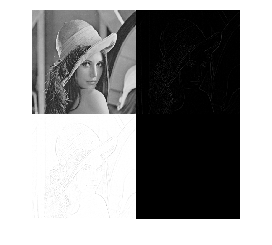
Binarization of the DoG result to highlight significant edges

After computing an edge or scale-difference response, it is often necessary to decide which responses are important enough. Binarization makes this selection with a threshold: strong values are kept and weak values are removed. This makes the result easier to interpret as a set of candidate edges.

lena_dog = lena_dog > 5;

lena_dog_negativa = lena_dog_negativa < 250;

montage({lena,lena_dog,lena_dog_negativa})